Em analyzes 3-D structures embedded in planar multilayered dielectric on an underlying fixed grid. For this class of circuits, em can use the FFT (Fast Fourier Transform) analysis technique to efficiently calculate the electromagnetic coupling on and between each dielectric surface. This provides em with its several orders of magnitude of speed increase over volume meshing and other non-FFT based surface meshing techniques.
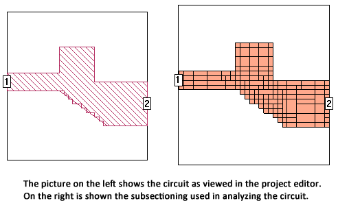
Em is a complete electromagnetic analysis; all electromagnetic effects, such as dispersion, loss, stray coupling, etc., are included. There are only two approximations used by em. First, the finite numerical precision inherent in digital computers. Second, em subdivides the metalization into small subsections made up of cells.
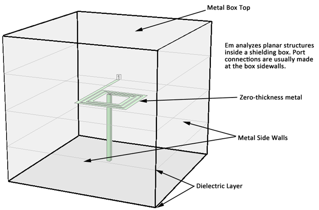
Em performs an electromagnetic analysis of a microstrip, stripline, coplanar waveguide, or any other 3-D planar circuit by solving for the current distribution on the circuit metalization using the Method of Moments. The metalization is modeled as zero-thickness metal between dielectric layers.
Em evaluates the electric field everywhere due to the current in a single subsection. Em then repeats the calculation for every subsection in the circuit, one at a time. In so doing, em effectively calculates the “coupling” between each possible pair of subsections in the circuit.
Each subsection generates an electric field everywhere on the surface of the substrate, but we know that the total tangential electric field must be zero on the surface of any lossless conductor. This is the boundary condition: no voltage is allowed across a perfect conductor.
The problem is solved by assuming current on all subsections simultaneously. Em adjusts these currents so that the total tangential electric field, which is the sum of all the individual electric fields just calculated, goes to zero everywhere that there is a conductor. The currents that do this form the current distribution on the metalization. Once we have the currents, the S‑Parameters (or Y- or Z-) follow immediately.
If there is metalization loss, we modify the boundary condition. Rather than zero tangential electric field (zero voltage), we make the tangential electric field (the voltage on each subsection) proportional to the current in the subsection. Following Ohm’s Law, the constant of proportionality is the metalization surface resistivity (in Ohms/square).