Another very useful feature of the netlist project is the ability to insert modeled elements into a geometry project after an electromagnetic analysis has been performed on that circuit. A modeled element is an ideal element such as a resistor, inductor, capacitor or transmission line, which has a closed-form solution. No electromagnetic analyses are performed on modeled elements.
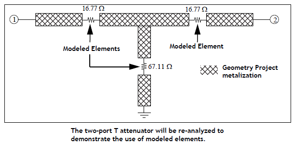
To demonstrate the use of modeled elements, we will again analyze the T attenuator. However, instead of the attenuator being the result of connecting the results of electromagnetic analyses as shown previously in A Network File with Geometry Project, in this case, the geometry project, att_lgeo.son, has the full attenuator with cutouts where the modeled elements need to be inserted. The three resistors will not be analyzed as part of the geometry project, but will be inserted as modeled elements in the netlist. The figure below shows the circuit layout with the modeled resistor elements. A geometry project for the transmission line structures is created first. A netlist project will then be used to insert the three resistors and calculate two-port S-parameters for the overall circuit.
To accomplish this task, it is necessary to create a geometry project with the transmission line structure and three “holes” where modeled elements will eventually be inserted. The figure below shows such a geometry project. Here, pairs of co-calibrated ports have been placed on the edges of each modeled element “hole”. Co-calibrated internal ports are identified as a calibration group with a common ground node connection and a defined terminal width. When em performs the electromagnetic analysis, the co-calibrated ports within the group are simultaneously de-embedded. When the modeled elements are inserted later on, each is connected across the corresponding pair of co-calibrated ports. Note that under certain conditions, delta gap ports can be used instead of co-calibrated ports. See Using Delta Gap Ports for details.
Below is the netlist, att_lumped.son, that will be used for this example.
The netlist above instructs em to perform the following steps:
The two projects, att_lgeo.son and att_lumped.son are available in the Att example for Netlist Project Analysis.
The listing below is the analysis output as it appears in the analysis monitor. Note that these results are similar to the results given above for distributed elements.