This section describes how to use Sonnet to analyze 3-D planar radiating structures, such as microstrip patch arrays.
Also, this chapter discusses the Far Field Viewer. The Far Field Viewer calculates and plots far field antenna patterns for arbitrary 3-D planar geometries. It uses the current distribution data in the project as input, and creates a pattern. The pattern may be viewed as a Cartesian or Polar plot.
NOTE: The Far Field Viewer feature is only available if you have purchased a Far Field Viewer license from Sonnet. The Far Field Viewer license is an optional add-on to Sonnet Suites and must be purchased separately.
Since em is an analysis of 3-D planar circuits in a completely enclosing, shielding, rectangular box, the analysis of radiating structures is not an application which immediately comes to mind.
However, if we can set up the project correctly, we can model many types of radiating structures using Sonnet. It is important to keep in mind that, unless the environment is carefully prepared, the analysis may yield incorrect results. The following list of conditions should be met in order to obtain accurate results.
First Condition: Make both of the lateral substrate dimensions greater than one or two wavelengths.
When modeling in an open environment, we view the sidewalls of the shielding box as forming a waveguide, whose tube extends in the vertical direction. This setup propagates energy from the antenna toward the top cover of the analysis box. Radiation is then approximated as a sum of many waveguide modes. If the tube is too small, there are few, if any, propagating modes, violating the First Condition.
When modeling radiation from small discontinuities, you can easily make a mistake. Discontinuities are usually small with respect to wavelength. To conduct a discontinuity analysis, place the sidewalls one or two substrate thicknesses from the discontinuity. If the sidewalls form below a cut-off waveguide, there is no radiation. In this case, the substrate dimensions are unlikely to meet the First Condition.
Second Condition: Make sure the sidewalls are far enough from the radiating structure that the sidewalls have no affect.
Another way to look at this condition is to consider the image of the structure (discontinuity or antenna) created by the sidewall. Position the sidewall so that the image it forms has no significant coupling with the desired structure.
Usually, two to three wavelengths from the sidewall is sufficient for discontinuities. For single patch antennas, one to three wavelengths is suggested. Requirements for specific structures can easily be greater than these guidelines. If the First Condition requires a larger substrate dimension than the Second Condition, it is very important that the larger dimension is used.
If you are using the Far Field Viewer, the larger the box the better. The Far Field Viewer assumes that S-parameters from em are from a perfect open environment. If some of the power is reflected because a box is too small, the input power calculated by the Far Field Viewer will be slightly incorrect. The Far Field Viewer then calculates antenna efficiencies greater then 100%. If this occurs, the box size should be increased.
Third Condition: Place the top cover outside the fringing fields (i.e., near field) of the radiating structure, preferably a half wavelength.
The position and distance of the top cover is important. This condition is violated when the resistive top cover becomes involved in the reactive fringing fields which form the near field of the radiator. In turn, this changes what would have been reactive input impedance into resistive input impedance, overestimating the radiation loss.
Do not place the top cover thousands of wavelengths away from the radiator. Extreme aspect ratios of the box should be avoided. Empirical data for patch antennas has shown, that a distance of about 1/2 wavelength works best.
Fourth Condition: Set the top cover to Free Space.
This value is a compromise. All TE modes have a characteristic impedance larger than 377 ohms, while all TM modes are lower. Thus, while a 377 Ohms/square top cover does not perfectly terminate any mode, it forms an excellent compromise termination for many modes. This approximates removing the top cover of the box. As the analysis box size increases, both the TE and TM lower order modes approach 377 ohms. Thus, the larger the box, the better the approximation.
Fifth Condition: The radiating structure can not generate a significant surface wave.
If there is a significant surface wave, it is reflected by the sidewalls of the box.Unless this is the actual situation, such antennas are inappropriate for this technique. Actually, the Fifth Condition is a special case of the Second Condition, since if there is significant surface wave, the Second Condition cannot be met. This condition is stated explicitly because of its importance.
In general, any surface wave is both reflected and refracted when it encounters the edge of the substrate. This boundary condition is different from either the conducting wall of Sonnet or the infinite substrate provided by a true open space analysis.
A dual patch antenna is illustrated conceptually below.
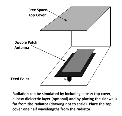
The feed point is created in the project editor by creating a via to ground at the feed point. Then the ground end of that via is specified as a port, just as one would specify a more typical port on the edge of the substrate at a box sidewall. A file showing an antenna similar to this one is named “stackedpatch.son” and is available in the Sonnet examples.
The purpose of the Far Field Viewer is to calculate the far field pattern of an antenna for a given excitation and set of directions. In Sonnet we use phi and theta ranges. The Far Field Viewer reads the current density data generated by em for the antenna at the desired frequencies. Then it imports the current distribution information into the project and generates the desired Far Field antenna pattern information. A default set of values for port excitations and terminations are used to calculate plots for the first frequency upon start-up of the Far Field Viewer. Thereafter, the user specifies the frequencies and angles for the radiation pattern and the desired port excitations and terminations.
Since the Far Field Viewer uses the current density data generated by em, it can analyze the same types of circuits as em. Some of these circuit types include microstrip, coplanar structures, patch antennas, arrays of patches, and any other multi-layer circuit. As with em, the Far Field Viewer can analyze any number of ports, metal types, and frequencies. However, the Far Field Viewer cannot analyze circuits that radiate sideways. These include structures with radiation due to vertical components, coaxial structures, wire antennas, surface wave antennas, ferrite components, or structures that require multiple dielectric constants on a single layer.
Be aware that although the current data is calculated in em with a metal box, the metal box is removed in the Far Field Viewer calculations. The modeling considerations discussed earlier in the chapter are important. However, the accuracy of the Far Field Viewer data relies on the accuracy of the em simulation.
The Far Field Viewer has the following limitations:
1. The plotted antenna patterns do not represent de-embedded data. Therefore, the effect of the port discontinuity is still included even if you specify de-embedding when running em.
2. Radiation from triangular subsections (i.e., diagonal fill) is not included.
3. The Far Field Viewer patterns are designed for a substrate which extends to infinity in the lateral dimensions.
To view an antenna plot, the Far Field Viewer uses the spherical coordinate system shown below. The X, Y, and Z coordinates are those used in the analysis engine, em, and the project editor. The XY plane is the plane of your project editor window, with the Z-axis pointing toward the top of the box. The spherical coordinate system uses theta (θ) and phi (ϕ) as shown in the figure below.
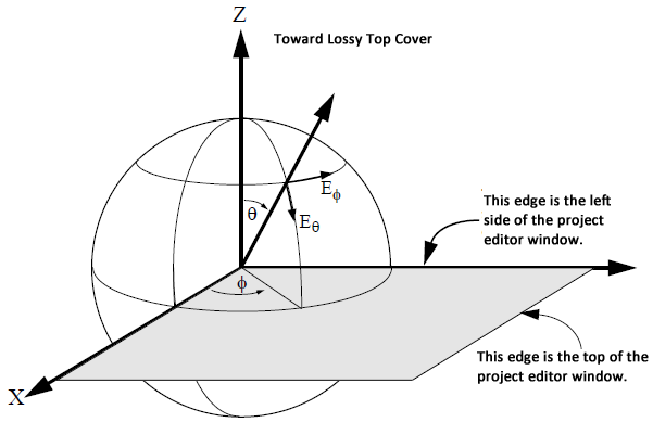
This spherical coordinate system allows values for theta from 0 to 180 degrees. However, values of theta greater than 90 degrees are below the horizon, and are only useful for antennas without infinite ground planes. To view the top hemisphere, sweep theta from 0 to 90 degrees and sweep phi from -180 to +180 degrees.
The X and Y axes in the figure above correspond to the X and Y axes in the project editor. The origin is always located in the lower left corner of the project editor window.
To look at an E-plane cut or an H-plane cut, set phi (ϕ) to 0 or 90 degrees, and sweep theta (θ) from 0 to 90 degrees. To view an azimuthal plot, set θ and sweep ϕ.
NOTE: The Far Field Viewer will allow the user to analyze the same space twice with the user determining the appropriate angle ranges for each analysis. For details, see Graph - Calculations in the Far Field Pattern Tab.
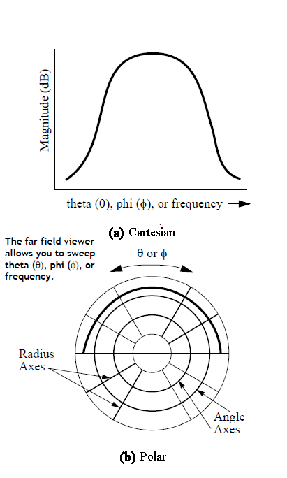
The Far Field Viewer displays two plot types: Cartesian and polar. Both types of plots are shown below. The Cartesian plot allows the magnitude (in dB) to be plotted on a rectangular graph with your choice of theta (θ), phi (ϕ), or frequency for the X-axis as shown in the figure below. The polar plot allows you to select either theta (θ) or phi (ϕ) for the angle axis.
Selecting Graph - Graph Options - Normalization from the Far Field Pattern Tab main menu allows you to select the type of normalization to use for your plot. Once a normalization type is selected, all curves use that normalization.
You may choose between three types of normalization: Power Gain (dB), Directive Gain (dB), or Power/EMC. By default, the Far Field Pattern Tab displays the Gain (dB). You select the type of normalization by clicking on the appropriate radio button.
Power Gain (dB)
The power gain is defined as the radiation intensity divided by the uniform radiation intensity that would exist if the total power supplied to the antenna were radiated isotropically.1
Include Reflection: Select this checkbox to base the gain calculation on the total available power at the source rather than the total power delivered to the load.
Directive Gain (dB)
Directive gain is defined as the radiation intensity from an antenna in a given direction, divided by the uniform radiation intensity for an isotropic radiator, with the same total radiation power.2
The Far Field Viewer calculates the directive gain based on the total power radiated by your circuit. It calculates the total power by using all the theta (θ) and phi (ϕ) points to integrate over the entire surface. Therefore, the more theta and phi points calculated, the more accurate the values are provided for the directive gain. A Figure of Merit (F.O.M.) appears in this dialog box and in the normalization panel when directive gain is selected to provide you with an idea of the accuracy of the data (100% is perfect). If this figure is too low, try recalculating it using more theta and phi points. If this figure is too high, it is an indication that the problem is over calculated. i,e, angles are being analyzed twice. In this case, check for duplicate angles such as theta = 180 and theta = -180.
Power/ EMC
Selecting the Power/ EMC for the normalization displays the power at a given angle.
Absolute Unit: You may display the power in Watts/ Steradian, Volts/Meter at a distance of 3 M and Volts/Meter at a distance of 10 M.
Relative to setting
This section is only available for Power Gain and Directive Gain normalizations.
Relative to: A reference point from which the gain is calculated. The choices are:
- Isotropic: Normalizes the data to a theoretical isotropic antenna in free space.
- Arbitrary: Normalizes the data to an arbitrary value which you enter in the Reference Value text entry box.
Reference Value: The value provides the reference point in dB for the normalization when using the arbitrary setting.
The Far Field Viewer displays the magnitude of the electric field vector for a given direction. The magnitude may be represented as the vector sum of two polarization components, E-theta (Εϕ) and E-phi (Εθ) as shown in the figure describing spherical coordinates shown below.
The Far Field Viewer allows you to see the total magnitude or either component of the magnitude. Other polarization results are also available in the Far Field Viewer and are discussed in the Measurement Section
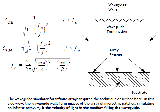
Em can be used to simulate infinite arrays using a waveguide simulator. In this technique, a portion of the array is placed within a waveguide. The waveguide tube is vertical, connecting the radiating patches to the termination, which is a matched load. The images formed by the waveguide walls properly model the entire infinite array scanned to a specific angle.
The sidewalls of the shielding box in the em analysis easily represent the sidewalls of the waveguide in the infinite array waveguide simulator. A side view is shown below.
Providing a termination for the end of the waveguide requires a little more thought. Any waveguide mode can be perfectly terminated by making the top cover resistivity in em equal to the waveguide mode impedance. This can be done in the project editor automatically at all frequencies and all modes by selecting "WG Load" from the metals in the Top Metal drop list in the Box Page of the Circuit Settings dialog box (Circuit - Settings).
In a phased array with the array scanned to a specific direction, a single waveguide mode is generated. The em software can model the waveguide simulator of that infinite array just by setting the top cover impedance to the impedance of the excited waveguide mode.
1Simon Ramo, John R. Whinnery and Theodore Van Duzer, Fields and Waves in Communication Electronics, John Wiley & Sons, Inc. 1994, pg. 601.
2Ibid, pg. 600.