N-Coupled Line Model
Most circuit design programs provide models for single and multiple-coupled transmission lines. However, it is often desirable to use EM simulated data in circuit design programs. These programs often provide transmission line models which utilize RLGC parameters. R, L, G, and C are the resistance, inductance, conductance and capacitance per meter of a transmission line. The RLGC parameters can be extracted from an EM simulation of a short section of the transmission line. They can then be used to model any length of line having the same cross-section.
Sonnet can create the RLGC parameters in a format compatible with the mtline component in Cadence Virtuoso Spectre and the W-element in Synopsis HSPICE.
Project Setup
Shown below is an example of a project composed of four transmission lines.
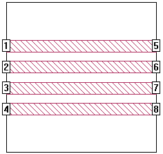
As in the circuit shown above, the input and output ports of the ith transmission line, Pin(i) and Pout(i) respectively, must be numbered as follows:
- Pin(i) = i
- Pout(i) = i + N
where N is the total number of lines.
The equivalent circuit is shown below for the four transmission lines shown above. Some elements, such as capacitance values between non-adjacent lines and mutual inductances are not shown for clarity purposes.
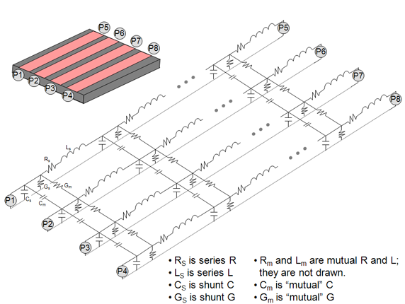
The N-Coupled Line Model requires the length of transmission line to be less than a half wavelength at your highest frequency. If the line is longer than a half wavelength, you may use reference planes to decrease the effective length. Reference planes are a property of a port and are discussed in detail in Shifting Reference Planes.
Creating the Model File
There are two methods you may use to generate an N-Coupled Line Model file:
Automatic: You may set up your project so the EM solver will automatically generate a N-Coupled Line Model file. From the Project Editor, select Circuit > Settings > [Output Files] and then select Add File > N-Coupled Line Model.
Interactive: After simulating your project, you may generate the file from a Sonnet graph. Select a curve representing the desired project, and then select Output > N-Coupled Model File.
You may obtain a short description for each option by hovering your mouse over the option in any dialog box.
interpreting the Results
The output file contains four matrices: one for the inductance, one for resistance, one for capacitance, and one for conductance. For a single transmission line, each matrix is a 1x1 matrix, so each matrix is a single value. Since the matrix is symmetrical, identical values are not reported. For example, for two transmission lines, each matrix is a 2x2 matrix, but the file contains only three values per matrix because the matrices are symmetrical.
The order and format of the matrices is given in the comments of the output file. The inductance and resistance matrices are straightforward; i.e., they represent the self and mutual inductance and resistance per meter. However, the capacitance and conductance matrices use "Maxwell" format:
- The off-diagonal elements represent the negative of the mutual capacitance and conductance per meter.
- The diagonal elements represent the self capacitance or conductance per meter minus the mutual values for that line.
Artificial Transmission Lines
The topic Z0 and Eeff explains how the EM Solver calculates the characteristic impedance and effective dielectric constant of a transmission line whose cross section does not change along the length of the line. However, designers may create artificial transmission lines which imitate the behavior of a transmission line over a limited frequency band. Some examples of artificial transmission lines include:
- Transmission lines with a patterned ground
- Periodically loaded transmission lines
- A repeating pattern of lumped inductors and capacitors
- Metamaterial slow-wave transmission lines
These transmission lines may be simulated in Sonnet but, as explained in the Z0 and Eeff topic, the characteristic impedance (Z0) and effective dielectric constant (Eeff) from the EM Solver will not accurately represent the artificial transmission line's Z0 and Eeff. Instead, you may use the N-Coupled Line model and view the comments of the file. The Z0 and Eeff are included in the comments.
An artificial transmission line example, called slow-wave, may be obtained using the Example Browser.