Z0 and Eeff
When your circuit is de-embedded, the characteristic impedance (Z0), and the effective dielectric constant (Eeff) of the transmission line connected to the port are calculated for each port. These values are calculated for all port types except ports with diagonal reference planes, ports which share a reference plane, and Via ports.
For ABS sweeps, Z0 and Eeff are calculated only for discrete frequencies. These values are not calculated at synthesized data points.
It is important to note that calculating Z0 and Eeff is based on the calibration standard used for de-embedding. For Box-wall ports, the calibration standard, as discussed in Calibration Standards, is based on a cross section of any polygon(s) touching the box wall that the port under consideration is on. This cross section is extended the length of the calibration standard. Since the cross section is taken at the box wall, the interior of the circuit does not affect the calculation.
In the example shown below, there is a single feedline connected to Port 1, with no metal on another level. Therefore, the transmission line upon which the calculation is based is reasonable and the resulting values are accurate.
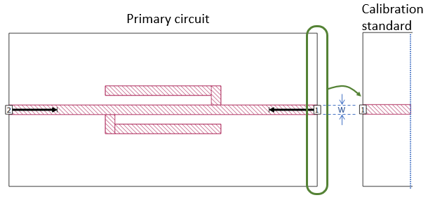
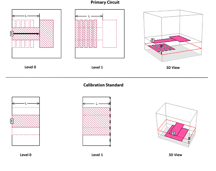
In the second example shown below, the primary circuit includes a metal pattern on Level 1, underneath the transmission line. Since the calibration standard is based on the primary circuit cross section at the box wall, it only contains the first polygon from the pattern. The length of the calibration standard matches the port 1 reference plane length in the primary circuit. The resulting Line Z0 and Line Eeff values are computed using a solid ground plane, instead of the periodic pattern in the primary circuit.
In addition, notice that the reference plane violates the rule discussed in Reference Planes Longer than the Feedline.
Please see the N-Coupled Line Model help topic for information on how to extract the Z0 and Eeff values for a the above case and other artificial transmission lines.
Lengths at Multiples of a Half-Wavelength
Eeff and Z0 are not available when the length of the calibration standard is near a multiple of a half wavelength. Note, however, that while the EM solver is unable to determine Eeff and Z0, all other results are still valid.
Lengths Much Greater than One Wavelength
If the length of the calibration standard is greater than one wavelength, incorrect Eeff values might be seen. However, all of the other results are still valid.
The EM solver calculates Eeff using the calibration standard phase data. At a given frequency and unwrapped phase value, the solver is not initially aware if the phase data has already passed through one or more 360 degree transitions. For example, the ANG[S21] data might be 5 degrees which means the actual calibration standard length could be 5, 365, 725 degrees, etc. The solver uses an iterative technique to determine the actual phase of the calibration standard. It first calculates Eeff based on the direct phase value, which in this example is 5 degrees. If this results in a non-physical Eeff value, it automatically adds 360 degrees to the phase value and again checks the Eeff value. If necessary, it repeats this step until a physical value (i.e., Eeff ≥ 1.0) is achieved.
This iterative procedure demonstrates that there is wide range of calibration standard lengths and phase values that are acceptable to extract the Eeff data. It is rare but the Eeff calculation can fail with extremely long calibration standard lengths. When this occurs, the Eeff value will drop to a value just above 1.0. The Z0 and other de-embedded results are still valid.
Graphing Z0 and Eeff
You can plot Z0 and Eeff as a function of frequency or parameter.
Frequency Sweep
When you wish to determine the transmission line parameters, Z0 and Eeff, you should:
Analyze a short length of transmission line as a one-port or two-port.
The electrical length of line should be greater than a few degrees and less than a half wavelength. The optimal length is a quarter wavelength. It is not recommended that you use an ABS sweep, since the Z0 and Eeff data is only calculated for the discrete data points. You should use Box-wall ports for the best results.
Select Launch > Graph Response > New Graph.
A new graph tab is opened. By default, dB[S11] is displayed.
Select Graph > Manage Curves.
The Manage Curves dialog box is opened.
In the Measurement section, click Line Z0 or Line Eeff.
Click Close.
A curve representing Z0 vs frequency or Eeff vs frequency is added to your graph.
Parameter Sweep
It is possible to plot Z0 or Eeff as a function of a variable used in your circuit. For example, you could plot Z0 vs line width using a Dimension Parameter for the width of a transmission line. The procedure for doing so is provided below.
Add a dimension parameter to vary the line width.
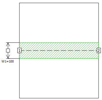
A symmetric dimension parameter would work best with this circuit since it uses symmetry. The circuit is shown below with a symmetric dimension parameter, W1, added. For more information about dimension parameters and how to add them to your circuit, please see Dimension Parameters.
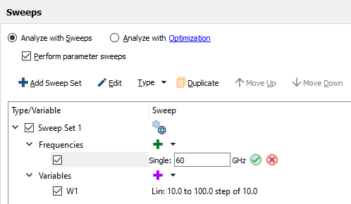
Set up a parameter sweep.
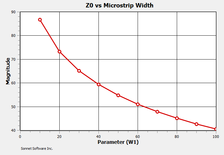
For this example, the circuit will be analyzed using a parameter sweep, varying the width of the line from 10 microns to 100 microns in steps of 10 microns at a single frequency of 60 GHz.
Analyze the project and graph the results.
A graph may be opened by clicking on the Graph icon in the Job Queues tab or selecting Launch > Graph Response from the main menu of the Project Editor tab or the Job Queues tab once the analysis has completed.
Select Graph > Plot Over > Parameter from the main menu of the Graph tab.
This changes the x-axis to be the parameter W1. If the project has more than one swept parameter, the x-axis will be the first one in the list, but this can be changed in the Manage Curves dialog box later.
Select Graph > Manage Curves from the main menu of the Graph tab.
The Manage Curves dialog box appears on your display.
Select Line Z0 under Transmission Lines in the Measurement panel.
This will plot the characteristic impedance of the transmission line connected to the selected port. The Properties panel is updated with the properties of the Line Z0 measurement. For this example, we will plot the magnitude of Z0 for Port 1, so no change needs to be made to the properties. If there were more than one frequency available, or if you swept more than one parameter, you would have needed to double-click on the Parameters field and selected the frequencies you wished to plot and the parameter over which you wanted to plot.
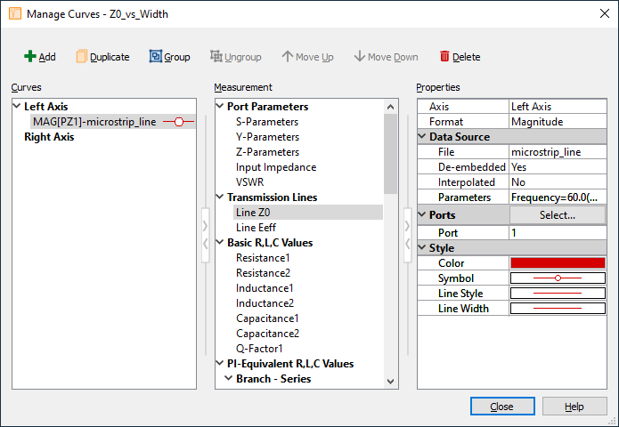
Click the Close button to close the Manage Curves dialog box.
The plot shows the magnitude of the characteristic impedance of the transmission line connected to Port 1 as a function of line width. The characteristic impedance decrease as the line gets wider. If you wished to plot Eeff, you would have chosen Line Eeff from the Measurement list.
Coupled Transmission Lines
If you have more than one port on a box wall, Z0 and Eeff cannot be determined as there is more than one mode for the transmission line. In this case, your output log will contain the words "Coupled Port" indicating that there are multiple ports. Even though Z0 and Eeff cannot be determined, the rest of the results are still valid.
For two symmetrical coupled lines, Sonnet can be used to compute the common and differential mode Z0 and Eeff values. The common and differential mode are very similar to the even mode and odd mode used by popular transmission line couplers (see Interpreting Z0 and Eeff). To create a project which can be used to find any of these quantities, start with a four-port coupled line circuit like the one shown below.
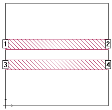 Notice that the lines are placed precisely in the center of the box. This is not necessary in many cases, but we suggest you do this to force the symmetry between the two lines.
Next, renumber your ports as shown below. The left two ports (+1/-1) represent the differential, or odd mode. The right two ports (+2/+2) represent the common, or even mode.
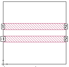 To renumber a port, right-click on the port and select Port Properties. This opens the Port Properties dialog box where you can change the port number.
Interpreting Z0 and Eeff
There is a subtle difference between the even/odd mode and common/differential mode Z01. Sonnet computes the common and differential mode Z0 values, but you can easily calculate the even and odd mode Z0 values by either multiplying or dividing the Sonnet results by two as shown in the equations below.
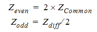 For example, if Sonnet reports a differential mode Z0 of 90 ohms, the odd mode Z0 is about 45 ohms. And if Sonnet reports a common mode Z0 of 28 ohms, the even mode Z0 is 56 ohms. The Eeff values do not need to be modified.
"Characterization of differential interconnects from time domain reflectometry measurements" by A. Tolescu and P. Svasta