Purpose
In this document, we will discuss efficient meshing in Sonnet, based on a wide variety of application examples. It will be shown how manual changes to the mesh can be applied that save memory and analysis time.
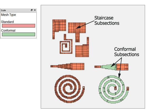
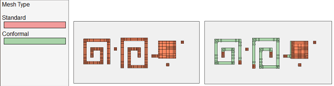
Meshing basics: staircase and conformal subsections
Based on the cell size, which is defined by the user, Sonnet will sample all geometries and divide them into pieces for analysis (“create a mesh”). The resulting mesh elements are called subsections. The main subsection types in Sonnet are staircase subsections and conformal subsections. Staircase subsections are rectangular subsections, which are parallel to the Sonnet analysis box walls and can have a linear current gradient in the x and/or y direction.Conformal subsections offer more degrees of freedom: their shape and orientation follow the underlying polygon, and the current on a conformal subsection has more degrees of freedom compared to a staircase subsection. This is more efficient for polygons with a curved or irregular shape. However, conformal subsections can only be applied to polygons which are transmission-line-like, i.e. the width is small compared to the wave length.
If you are familiar with other planar EM solvers, you might think that conformal subsections are similar to the triangular subsections used in those tools. That is not true, however, because those triangular subsections have very limited degrees of freedom for the current flow, similar to the Sonnet staircase subsections. The conformal subsections in Sonnet are much more powerful, as we will see.
By default, Sonnet uses staircase subsections for all metal, except for vias which use special via subsections. For each metal object (polygon), the meshing properties can be set in the object’s properties dialog shown below. If the object is not suitable for conformal meshing, the analysis engine will ignore the subsection type setting and switch back to staircase meshing for this object.
A third subsection type, called "Diagonal," is very similar to staircase subsections, but is rarely used. See Diagonal Fill Subsectioning in the Sonnet User's Guide for more information.
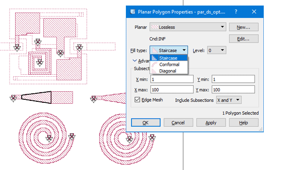
When Sonnet is used from the Keysight interface or Cadence interface, then a global fill type is set in the interface. This setting is applied to all polygons. To assign individual fill types to different polygons, it is necessary to open the simulation model in the Sonnet project editor.
When to use which fill type?
Staircase mesh is most efficient for rectangular polygons which are parallel to the box wall. Conformal mesh is more efficient for diagonal lines and geometries which are curved, or not parallel to the box walls.
Examples where staircase mesh is most efficient:
Examples where conformal mesh can be used for more efficient analysis:
Examples where staircase mesh should be used, and conformal mesh will be either inefficient or inaccurate:
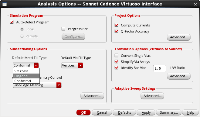
When you are using Sonnet from the ADS or Cadence interface, and you have to set one fill type for the complete layout, you can choose conformal mesh as your default. The software should then detect critical areas, and use staircase mesh where conformal mesh is not possible.
Why is analysis more efficient with conformal mesh for some circuits, and more efficient with staircase mesh for other circuits?
The Sonnet analysis consists of two parts: matrix fill and matrix solve. In the matrix fill part, we put current on one subsection, and calculate the induced voltage on all other subsections. We repeat this for all N subsections, and in the end, we have a coupling matrix with N*N elements. Then, the next step is matrix solve, where the matrix is inverted to calculate the port voltages. The memory requirement for the matrix is ~N2, and the time to invert the matrix is something like ~N3. This is the reason why matrix solve is the most time consuming part of the analysis when we have many subsections.
If the simulation model uses only staircase subsections, which have a relatively simple current distribution on each subsection, then the matrix fill calculations are fast and easy. However, the mesh might consist of many staircase subsections, so that we end up with a large matrix and long matrix solve time.
This had been a problem for applications like circular spiral inductors, where a staircase mesh creates a very large number of subsections. The memory requirement and analysis time were hardly acceptable. To solve this problem, the concept of conformal subsections was introduced.
A conformal subsection gives more degrees of freedom to the current on the subsection (technically: more complex basis functions), so that curved geometries can be described with a relatively small number of conformal subsections. This helps to reduce the matrix size and matrix solve time, because the number of subsections is much reduced. However, the matrix fill time is increased, because it is more complicated to calculate the coupling for conformal subsections. In other words, the choice of staircase vs. conformal subsections has to do with the balance between matrix fill time and matrix solve time. If matrix solve time is the bottleneck, then it makes sense to check if the number of subsections can be reduced by using conformal mesh for diagonal or curved polygons.
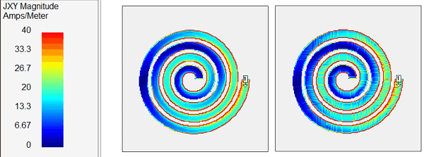
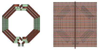
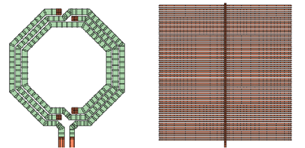
Spiral inductor meshing example
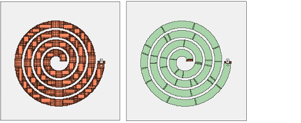
This example shows the benefit of conformal meshing for curved lines.
Staircase (Left) |
Conformal (Right) |
|
Number of subsections |
10612 |
520 |
CM Cell |
- |
52K |
Memory Required |
862 MB |
6 MB |
Matrix Fill Time |
- |
About 10% longer |
Matrix Solve Time |
2000X improvement |
|
Total Analysis Time |
11.5X Improvement |
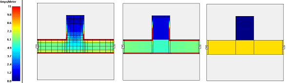
In the resulting current density, you can see that the conformal mesh analysis (right) has some more “grain” in the current distribution, but all relevant effects like high edge current and current crowding are represented within the conformal mesh subsections. Each conformal subsection has much internal current detail.
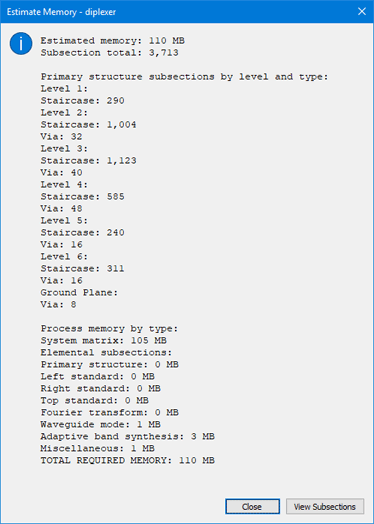
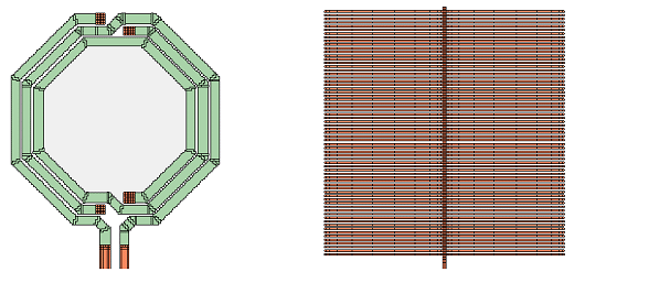
LTCC diplexer meshing example
This example shows an LTCC diplexer which consists of rectangular shapes only, so that it is perfectly suited for staircase meshing. Just for comparison, it has been analyzed with staircase mesh (left) and with conformal mesh (right).
Staircase (Left) |
Conformal (Right) |
|
Number of subsections |
3000 |
2754 |
CM Cell |
- |
10K |
Memory Required |
71 MB |
60 MB |
Matrix Fill Time |
- |
2X increase |
Matrix Solve Time |
- |
About 10% faster |
Total Analysis Time |
1.6X increase |
Here, we can see that the analysis was actually slowed down by using conformal meshing, which increased the matrix fill time. We can also see that in the proximity of vias, and for the big capacitor plates, the analysis engine switched from conformal mesh to staircase mesh.
Using conformal meshing for this layout is possible, but staircase meshing is more efficient.
How can I check the required memory and the mesh?
If you are working from the Sonnet project editor, use the menu item Circuit ⇒ Estimate Memory. If you are working from the ADS or Cadence interface, use the menu item Sonnet ⇒ Analysis ⇒ Estimate Memory.
This brings up a window that gives detailed mesh information: The amount of memory required, and how many subsections are required. The subsection count is also listed in detail per layer, so that you can identify layers with excessive subsection count.
From here, you can press the “View Subsections” button to bring up the graphical subsection display. You can use the up/down cursor keys to move between layers.
For staircase mesh, the user can control the mesh density in a couple of ways.
At a given cell size, the Sonnet default is to create a dense mesh with small subsections on the edges (to account for high edge current), at vias and at discontinuities where other polygons overlap. This algorithm can be controlled by the user, globally for the entire model and also on a per-polygon basis. The global control for the mesh density is found in the EM Options page of the Circuit Settings dialog box (select Circuit ⇒ Settings from the project editor main menu, then select EM Options in the side bar menu of the Circuit Settings dialog box which appears on your display).
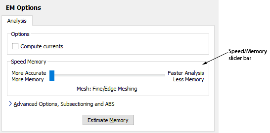
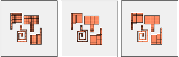
The EM Options page of the Circuit Settings dialog box allows you to set the global mesh density to three different levels: “More Accurate, More Memory”, “Faster Analysis, Less Memory” and a compromise between these two extremes. We will look in detail on the next page at what these settings mean. As an introduction, we have plotted the resulting mesh for these three settings below. The memory requirement is 93MB, 45MB and 22MB. The cell size is the same in all three cases.
So what does this mesh density mean? There is a good description in the Sonnet User’s Guide in Subsectioning. We will show the results here but for details, please refer to the Sonnet User’s Guide.
The image below shows the calculated current density of a line with an open ended stub, at the three different mesh density settings offered by the Speed/Memory control. Black lines show the subsection boundaries. All subsections are staircase. The analysis frequency of 100MHz is low, so that the maximum subsection size of 1/20 wavelength allows really large subsections for this comparison. At higher frequencies, the 1/20 wavelength limit would enforce smaller (and thus more) subsections for the coarse mesh case.
In the left current distribution, the fine mesh with many subsections gives the current the freedom to show important details: we have high edge current on the line, and the current starts to flow into the open ended stub at the corners, and then chooses a different path. With the medium setting, we loose some details, but overall, we get a similar behavior. In the right current distribution, with coarse mesh and big subsections without edge mesh, none of these effects is visible. There is only one (staircase) subsection across the width of the line, which means that the current must be constant over the width of the line. Also, we do not see any current entering into the stub, because the staircase subsection can only have one current gradient in y direction, and the sum of the current going into and coming out of the stub subsection is zero. As a result, that subsection has no current in the analysis result. It can be seen that all fine details are averaged out by the coarse mesh.
For real world analysis, the medium setting of the Speed/Memory slider is a fast and efficient way to reduce the mesh density of staircase subsections, and make the analysis run faster. The error from that less detailed mesh is acceptable in most cases (solvers such as Keysight Momentum use such a mesh as default). However, the right “Faster Analysis, Less Memory” will have a visible negative impact on accuracy in most cases, so that it should only be used for quick & dirty analysis, or if this is the only way to simulate a model when the computer has too little memory.
NOTE: The Speed/Memory slider has no effect on polygons with conformal mesh. It only controls staircase subsections.
Mesh density per polygon: xmin/ ymin and xmax/ ymax
So far, we have discussed the global mesh density setting with the Speed/Memory slider. In addition, when working from the Sonnet project editor, the mesh density of staircase subsections can be controlled individually for each polygon.
By default, Sonnet creates subsections which are 1 cell by 1 cell in the corner, and 1 cell wide along the edges. To the interior of the polygons, the size of subsections is gradually increased, each time doubling the subsection size, until it reaches the maximum size of 1/20 wavelength at the highest analysis frequency.
When you double click on a polygon, a dialog opens where the “Subsection Controls” are available for this polygon: minimum and maximum subsection size (in cells) and edge mesh.
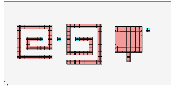
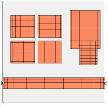
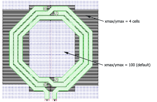
By using the xmin/ ymin settings, we can request bigger subsections than the global setting. To use these individual settings, the global Speed/Memory slider should be set to “More Accurate, More Memory.” We can then use the individual settings of the polygons to define a coarse mesh (big subsections) where appropriate. The image below shows an example of identical polygons with different xmin/ ymin settings. The rectangle on the top left side uses the default values (xmin=1, ymin=1) and the others use (xmin=2, ymin2) and (xmin=4, ymin=4) with and without edge mesh. A detailed description of these settings can be found in Changing the Subsectioning of a Polygon in the Sonnet User’s Guide.
Dummy polygons to locally control the mesh
By default, Sonnet refines the mesh at the polygon edges, and the mesh density can be controlled separately for each polygon. By using dummy polygons, it is possible to define regions with a different mesh inside other polygons. Sonnet will treat the dummy polygon as a separate object, so that we have all degrees of freedom related to the subsection settings.
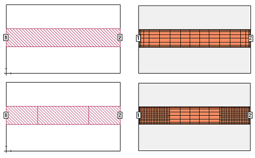
An example is shown below. The top two graphics show a simple through line in the project editor with the default subsectioning shown to the right. In the bottom graphics, the through line has been split into three polygons; electrically, the circuits are identical, but by using separate polygons, you may now use different controls for the subsectioning. Shown to the left of the project editor view, is the subsectioning with a finer mesh used for the outside “dummy” polygons.
Application example: Microwave filter
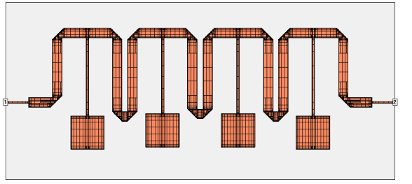
This example shows a superconducting microstrip filter. The width of the feedline is 160µm, the width of the narrow lines at the patches is 240µm. To obtain very high accuracy, the cell size was set to 40µm, so that we have 4 cells per line width for the narrowest line.
With such a small cell size, we get a dense mesh with the default settings. The default mesh takes 8644 subsections and 311MB of memory.
If we analyze with the Speed/Memory slider in the middle setting (large subsections with edge mesh), the mesh density is reduced to 3769 subsections and 81MB of memory. The analysis time per frequency is only 25% of the time required for the default mesh.
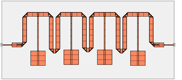
It is obvious that with the coarse mesh, some current details at the discontinuities cannot be represented as nicely, compared to the default mesh. Depending on the circuit, this may or may not be critical.
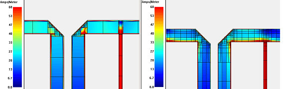
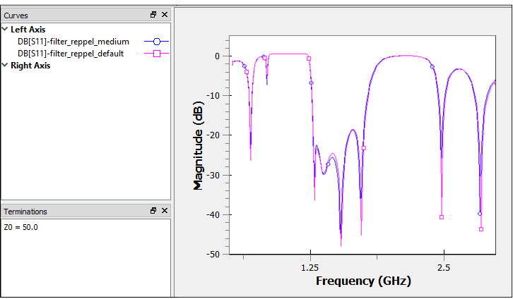
When we compare results, it can be seen that the two analysis results are very similar. This filter is not sensitive to the small errors in the current, so that the medium Speed/memory setting can be used during filter development. For final verification, when the design is ready, it might be good to double check results with the most accurate setting.
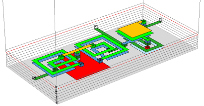
Application example: Compact UWB filter
This example of an electrically large structure is based on the following paper:
Compact Ultra-Wideband Microstrip/Coplanar Waveguide Bandpass Filter, Neil Thomson, Jia-Sheng Hong, IEEE MICROWAVE AND WIRELESS COMPONENTS LETTERS, VOL. 17, NO. 3, MARCH 2007
The filter comprises of a single CPW quarter wavelength resonator which is coupled to two microstrip open-circuited stubs on the other side of a common substrate. The images below show the upper and lower metalization layer.
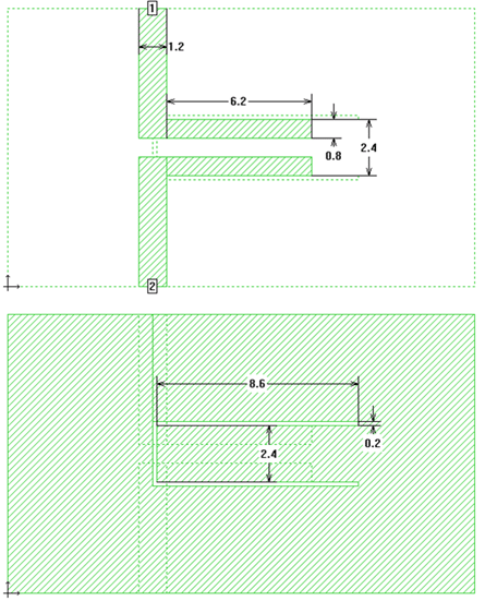
This application is of interest because we have a large amount of metal that must be meshed on the CPW side. Fortunately, all dimensions are a multiple of the slot width 0.2mm, so that we can do a first (fast) simulation with the cell size set to the slot size.
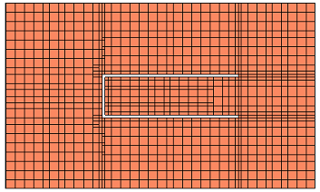
Many subsections are created because the structure is electrically large (multiple wavelengths at the highest analysis frequency) and the maximum subsection size is limited to lambda/20. This also means that our Speed/memory slider, which could enforce a more aggressive merging of subsections up to the lambda/20 limit, will not have much effect for this model at this cell size.
With the default settings, the number of subsections for this model is 2298 and the memory requirement is 45MB at 0.2mm cell size.
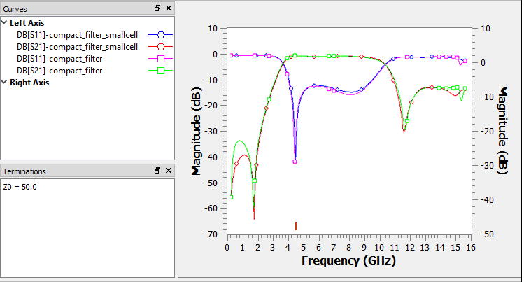
Now, we reduce the cell size from 0.2mm to 0.1mm and check the mesh and memory requirement again. As you can see from the mesh view below, there is almost no change in the areas which are far away from the slots: many subsections have the maximum size of lambda/20. At the slot, there are some additional subsections, giving a more accurate mesh there. With the default settings, the number of subsections for this model is 2500 and the memory requirement is 55MB at 0.1mm cell size. The analysis time increased but not by a significant amount.

In the results, there are some differences between 0.2mm and 0.1mm cell size. With the small difference in analysis time, it might be useful to run the analysis with the smaller cell size, for more accurate results. As described before, the Speed/Memory setting does not have much effect for this simulation model, so we leave it to the default (most accurate) setting.
Application example: Spiral inductor with ground shield
This example describes a spiral inductor with basic ground shield.
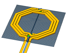
The inductor itself can be meshed with conformal subsections, and the ground shield with staircase subsections. However, the automatic mesh alignment between the layers might cause trouble here. That algorithm aligns the subsection boundaries of adjacent layers, which is good to ensure that the capacitance between the subsections is calculated with high precision. In our example, that creates a very dense staircase mesh on the ground shield, and reverts diagonal lines back to staircase on the inductor. The corresponding memory requirement is 2.7GB, and we will now apply manual changes for a more efficient mesh.
The setting that we change first is the detection of subsection boundaries. In the project editor, this is found in the Advanced Subsectioning tab in the EM Options page of the Circuit Settings dialog box.
The default value is 1, so that one layer above and below is checked for mesh alignment. This is a good value which makes sense in many cases. In some cases, we will increase that value, because we want the automatic subsection alignment across several layers (MIM capacitor with multiple dielectrics between the capacitor plates). However, in our case, we will set the value to 0 and care about the proper subsections ourselves.
If we set the polygon edge checking to 0 layers, without making further changes, the memory requirement is reduced to 135MB and we get a mesh like this:
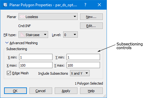
In order to get a more accurate capacitance between the inductor and the ground shield, we will now tweak the mesh manually, to get small subsections in those areas where the inductor and the ground shield overlap. The ground shield was cut (Edit ⇒ Divide) and then the subsection size was limited to xmax=4, ymax=4 for selected polygons, as shown below. This means that subsections will reach a maximum size of 4 cells in each direction. This setting is done in the polygon properties of the selected polygons. You can select multiple polygons, and then assign the values to all of them in one step.
Next, the subsection size is limited for the conformal mesh subsections. This setting is available in the Planar Polygon Properties dialog box (Object ⇒ Metal Properties) through the “Maximum length” parameter under Conformal Mesh Subsectioning Control. Note that this value is defined in length units, whereas the xmax/ ymax values are defined in multiples of the cell size.
A resulting mesh could look like this: short conformal subsections and small staircase cells in those areas where the inductor and the shield overlap, so that we get good results for the capacitance. With too large cells that are not aligned, the capacitance would he underestimated. The cells are still not aligned, but they are small enough now, so that the required current/charge can build up.
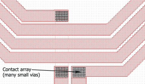
Application example: Spiral inductor with large contact array
For inductors with high Q factor, metal layers are often connected in parallel.
In the hardware, this might be realized by large contact arrays. These contacts will only allow a current flow between the metal layers (in z direction), and do not increase the effective cross section of the inductor itself. The large contact arrays do not change the resistance and quality factor of the inductor.
For this reason, the large contact array can be replaced by a small number of vias in selected places, every quarter turn or so. This applies to the hardware, and at the same time, is the recommended method to model parallel conductors in Sonnet.
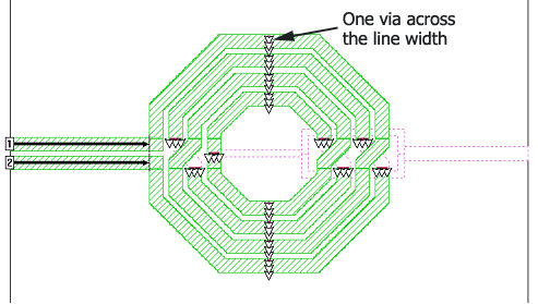
Having vias only in selected places helps Sonnet in multiple ways: conformal meshing is disabled close to a via. If the complete inductor is covered with vias, Sonnet will switch back to staircase subsections everywhere, and use a large amount of memory. Everything is more efficient if the vias are localized. Even the Sonnet editor will become slow when the models contains an excessive amount (thousands) of small vias.
A limited amount of contact arrays is acceptable, as shown in the example below. However, the contact arrays can be also be simplified and treated as one larger via by using a via metal type that uses the Array Loss model for the contact arrays. This via simplification can be done automatically when using our translators or interfaces, please see Via Simplification for more details.