You may also use variables to perform an optimization on your circuit. An optimization allows you to specify goals - the desired response of your circuit - and the data range for the variable(s) over which you seek the response. The software, using a conjugate gradient method, iterates through multiple variable values, searching for the best set which meets your desired goals.
The conjugate gradient optimizer begins by analyzing the circuit at the nominal variable values. It then perturbs each variable individually, while holding the others fixed at their nominal values, to determine the gradient of the error function for that variable. Once it has perturbed each variable, it then performs a line search in the direction of decreasing error function for all variables. After some iterations on the line search, the optimizer again calculates the gradients for all variables by perturbing them from their present “best” values. Following this, a new line search is performed. This continues until one of three conditions are met: 1) the error goes to zero 2) the error after the present line search is no better than the error from the previous line search 3) the maximum number of iterations is reached. When one of these three conditions is met, the optimizer halts.
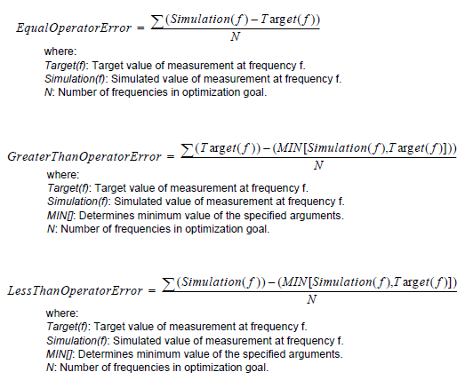
The equations used to determine the optimization goal error are as follows:
Setting up an optimization consists of five parts:
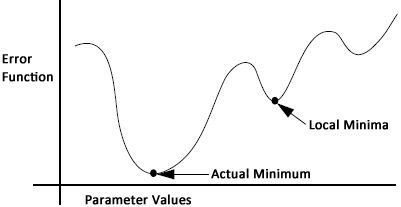
Care should be taken when setting the nominal values for the variables to be optimized. The optimizer starts at the nominal values and converges to the minima which is closest to those nominal values. Thus, it is highly recommended that you perform some pre-analysis prior to doing the optimization to ensure that the nominal values are in the right value range when the optimizer is started. Otherwise, the optimizer may converge to a local minima for which the error is not the minimum achievable value, as pictured below.
You specify a goal by identifying a particular measurement and what value you desire it to be. For example S11 < -20 dB. Keep in mind that the goals you specify may not be possible to satisfy. Em finds the solution with the least error. You may assign more priority to a goal by specifying a higher weight factor. For more details see Weight Factor below.
You may also specify a goal by equating a measurement in one network to a measurement in another network or file. For example, you may set S11 for network “Model” equal to S11 for network “Measured.” Likewise, you may equate S11 for network “Model” to S11 for data file “meas.s2p.”
You may select one or multiple variables to optimize. For each variable that you select you must specify minimum and maximum bounds. The analysis limits the variables to values within the specified bounds.
Variables that are used in an optimization have a granularity value assigned to them; the granularity defines the finest resolution, the smallest interval between values, of a variable for which em will do a full electromagnetic simulation during optimization. For values which occur between those set by this resolution, em performs an interpolation to produce the analysis data. By default, the software determines the granularity, but you may enter a value manually.
You specify the number of iterations. For each iteration, em selects a value for each of the variables included in the optimization, then analyzes the circuit at each frequency specified in the goals. Depending on the complexity of the circuit, the number of analysis frequencies and the number of variable combinations, an optimization may take a significant amount of processing time. The number of iterations provides a measure of control over the process. Note that the number of iterations is a maximum. An optimization can stop after fewer iterations if the optimization goal is achieved or it finds a minima (finds no improvement in the error in further iterations).
Once the optimization is complete, the user has a choice of accepting the optimal values for the variables resulting from the em analysis. Note that for dimension parameters, if the results of the optimization are accepted, the actual metalization in the project editor is the closest approximation which fits the present grid settings. As a matter of fact, em analyzes “snapped” circuits and interpolates to produce responses for circuits which do not exactly fit the grid. For more information about the grid, see Subsectioning.
If you have multiple optimization goals, the weight allows you to identify the priority of each goal for em, the analysis engine. The weight must be greater than zero. The higher the value, the higher the priority placed on the goal.
The equations used to calculate error, detailed above, take the absolute error and divide it by the number for frequency points, so it is finding an average error for the specified band. An error term is computed for each specified goal. If an optimization has more that one goal, the error terms are added together to compute the overall error term.
Before adding the error terms for the goals, each error term is multiplied by the goal's specified weight factor. If the weight factor is increased for a particular goal, it will increase the overall error term and that goal’s error will constitute a larger percentage of the overall error term. This is the mechanism by which weight factor prioritizes a goal.