Tutorial: Graph Your Results
In this part of the tutorial, you will create a graph of your project. You may graph Sonnet results as either a Cartesian graph or Smith chart by opening a Graph tab. For Cartesian graphs, you can graph S, Y, and Z-parameters and equations that are derived from the S, Y, or Z-parameters, such as inductance and Q-factor. Multiple projects can be plotted on a single graph, and S-parameter files from measurement systems can also be added to the same graph.
Open Example File
This page assumes you have already analyzed the project file part3_finalized.sonx. If you have not, you may use the example file provided with your Sonnet installation. Click the triangle below to expand the instructions for obtaining the example file.
Obtaining the Example FileObtaining the Example File
To obtain the example file, follow these instructions.
Select Help > Browse Examples from any Sonnet tab.
The Example Browser opens.
Find the Getting Started Tutorial and select it.
You may use the search box or scroll down until you see the Getting Started Tutorial example.
Click the Save button at the bottom of the Example Browser window.
A Save Example window opens with a list of files that will be saved.
Enter or browse for the folder where you wish to place the example files.
Choose a location you can remember.
Click the Save button.
The example files are saved to the specified folder.
Click the Close button.
The Example Browser closes.
If you have not done so already, open the file, part3_finalized.sonx by selecting File > Edit Project > Browse for File(s) from the main Sonnet Session tab.
Add/Modify Curves
In this tutorial, you will plot S11 in dB, then replace the S11 curve with an Inductance and a Q-factor curve.
Select Launch > Graph Response > New Graph.
A default graph of your project is opened in a new tab.
You may execute this command from the Project Editor tab or the Job Queues tab.
The default new graph is typically a graph of dB[S11]. However, you may change this behavior (see Graph and Pattern Preferences).
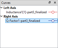
Select Graph > Manage Curves.
The Manage Curves dialog box appears. The left section contains the list of curves in your graph. Currently, it is a single curve (DB[S11]).
In the Curves section, select the DB[S11] entry.
After selecting a curve in the Curves section, selections made in the Measurement and Properties sections affect the presently selected curve. For example, changing the To Port from "1" to "2" in the Properties section changes the selected curve from DB[S11] to DB[S21].
In the Measurement section, select Inductance1, which is located under the Basic R,L,C Values category.
The Properties section is updated to reflect your selection, and the graph is updated with a curve of "Inductance1". You may need to move the Manage Curves dialog box to see the complete graph.
Sonnet provides multiple inductance measurements. "Inductance1" represents the inductance of your circuit, assuming a series RL. It is computed as follows:
For more information on inductance1, see Inductance1.
You may hover your cursor over any measurement for a brief description of the measurement. You may also right-click on it, and select Help on this measurement to open a longer description, including the equation used for the selected measurement.
Next, you will add a Q-factor curve to the right axis.
In the Curves section, select Right Axis.
Click the ![]() Add button on the Manage Curves toolbar.
Add button on the Manage Curves toolbar.
A new curve is added to the right axis. The default curve is DB[S11], so you will change it to Q-factor.
In the Measurement section, select Q-Factor1, which is located under the Basic R,L,C Values category.
The Properties section is updated to reflect your selection, and the graph is updated with a curve of "Q-factor1" on the right axis. Q-factor1 is computed as follows:
Click the Close button.
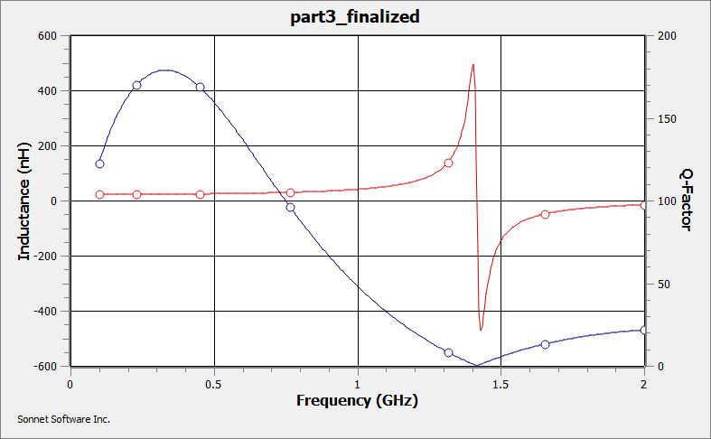
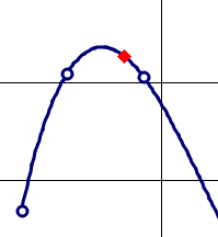
The Manage Curves dialog box closes. Your graph should look similar to the picture below:
Your Sonnet installation includes several graph templates of common graphs, including an L and Q curve template. To access these templates, select Graph > Apply Template. You can also create your own templates. See Graph and Pattern Templates for details.
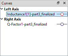
You may click the curve labels in the Curves Panel to highlight a specific curve as described in the next steps.
In the Curves panel, click the Inductance1 curve label.
The Inductance1 curve is highlighted.
In the Curves panel, click the Q-Factor1 curve label.
The Q-Factor1 curve is highlighted.
Obtaining Precise Data Point Values
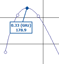
The graph shows that the maximum Q-factor occurs at approximately 0.3 GHz and the self resonance frequency is at approximately 1.4 GHz. The next steps demonstrate ways to obtain precise values on a graph.
Click anywhere on the Q-factor curve. The exact location is not important.
The point is highlighted and the status bar at the bottom of the graph displays the value of the selected data point.
Press the left and right arrow keys on your keyboard to move along the curve.
Each time you press one of the arrow keys, the status bar values change to reflect the newly selected point.
Right-click anywhere on the Q-factor curve and select Add Marker > Data Marker.
A Data Marker label appears and it moves with your cursor, waiting for you to position the label.
Move your mouse to position the marker label near the data point and click the mouse to pin the marker to that location.
A Data Marker and label are added to your graph. An example is shown below:
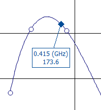
By default, the Data Marker label shows the frequency and value of the selected point. See Graph and Pattern Markers for information on customizing Markers.
Right-click on the newly added Data Marker and select Go To Max.
The marker moves to the maximum value of the curve and the Marker's frequency and Q-factor values are updated.
If the marker moves outside the graph, you may need to zoom out and drag it closer to your curve. To zoom out, you may use the middle mouse scroll wheel or the Zoom Out button on the toolbar.
To learn more about Markers, see Graph and Pattern Markers.
This concludes the graph tutorial. There are many more features not covered in this tutorial. If you would like to learn more about using Sonnet graphs, see Graphs - Overview. You may now close Sonnet, or, if you would like to view the current density of your circuit, you may continue by clicking the Next button below.