Adaptive Band Synthesis (ABS)
Introduction
The Adaptive Band Synthesis (ABS) technique provides results at a large number of frequency points by performing an EM analysis at only a small number of discrete frequencies. This technique provides a considerable reduction in processing time.
The EM solver performs the following steps for an ABS Sweep:
- The solver first performs a full EM analysis of the circuit at the start and stop frequencies storing extra internal data in a "cache" for each frequency analyzed.
- It continues solving at discrete points, adding to the cache data, and computing a rational polynomial fit to the data each time a new discrete point is added.
- This process continues until the EM solver determines that the rational polynomial fit has converged.
- Finally, it uses the converged polynomial to synthesize data at a large number of frequency points (approximately 300 points by default).
The EM solver dedicates the bulk of the analysis time to calculating the results at the discrete data points. Once the ABS sweep is complete, synthesizing data for the entire band uses a relatively small percentage of the processing time.
Setting up an Adaptive (ABS) Sweep
An Adaptive (ABS) Sweep is one of the frequency sweep types available when adding a sweep (see Edit/Add a Sweep). When you specify an ABS Sweep, you enter the start and stop frequencies in the two text entry boxes.
By default, the EM solver will synthesize approximately 300 frequency points between the start and stop frequencies. If you wish to increase or decrease this number, click the Settings icon  to the right of the controls. The appearance of the entry changes to display a target frequencies input field, where you may input the desired number of target frequencies. The actual number of data points will vary slightly from your target.
Using a small number of target frequencies does not speed up the analysis. Once a rational polynomial is found to fit the solution, calculating the adaptive data uses very little processing time. A really coarse resolution could produce bad results by not allowing the ABS algorithm to analyze at the needed discrete frequencies. A large number of target frequencies does not slow down the analysis unless the number of target frequencies is above approximately 1000 - 3000 points. It is recommended to use between 50 points and 2000 points.
Also, you may use the ABS technique to provide data for a Linear, Exponential, or Frequency List Sweep. If you select the Adaptive checkbox, Sonnet runs an Adaptive (ABS) sweep, then synthesizes the response at the requested frequencies.
DC Point Extrapolation
It should be noted that the EM solver cannot analyze at exactly DC because the coupling matrix becomes singular at DC. However, an ABS Sweep may be used to approximate a result at DC. To do this, enter a value of zero as the start frequency for an ABS Sweep. Once the ABS Sweep is complete the EM solver uses its polynomial fit to extrapolate to DC and provide an approximate result at DC.
Q-Factor Accuracy
By default, the ABS algorithm uses S-parameters as the criteria for convergence. The Q-Factor Accuracy run option adds the Q-factor of your analysis as a criterion for convergence. This results in a more accurate Q-factor but may require more discrete frequencies to be analyzed before convergence is reached.
To enable Q-Factor Accuracy using the Project Editor, follow these steps:
Select Circuit > Settings > [EM Options].
Click the Advanced drop-down arrow to display the advanced section.
You may skip this step if the Advanced section is already displayed.
Select the Configure ABS tab.
Select the Q-Factor accuracy checkbox.
Enhanced Resonance Detection
The Enhanced Resonance Detection feature is useful when your circuit response includes one or more extremely narrow band resonances that are typical for superconductor applications. When enabled, ABS searches for and resolves such resonances in detail by adding adaptive frequencies with very fine resolution in the vicinity of each resonance. The EM solver then performs an EM simulation at each detected resonance to obtain an extremely high level of accuracy in both magnitude and frequency. Although this results in higher accuracy, it requires more discrete frequencies to be analyzed before convergence is reached.
Approximately 300 additional synthesized data points are selectively added to the results around each resonance.
To enable Enhance Resonance Detection using the Project Editor:
Select Circuit > Settings > [EM Options].
Click the Advanced drop-down arrow to display the advanced section.
You may skip this step if the Advanced section is already displayed or if you are editing a netlist project.
Select the Configure ABS tab.
Skip this step if you are editing a netlist project.
Select the Enhanced resonance detection checkbox.
The example, supercond_resonators is an example project that uses Enhanced Resonance Detection and may be accessed using the Example Browser. See Enhanced Resonance Detection Example for a detailed discussion of this example.
ABS Caching Level
By default, the ABS cache is saved in your project after the job has finished. This can reduce processing time on subsequent ABS analyses. However, you may change the ABS Caching Level to prevent the cache from being saved. The three ABS Caching Levels are explained below.
None: Cache data is not retained. This option should only be selected if you have major constraints on disk space or if transferring data over a network takes a long time. If an ABS Sweep is stopped before the adaptive data has been calculated, you will have to start the analysis over from the beginning. Any processing time invested in the analysis is lost.
Stop/Restart: Retains the cache data while the analysis is proceeding. Once the adaptive data has been calculated, the cache data is deleted from the project. This setting provides for the circumstance in which the analysis is stopped or interrupted before the adaptive data is synthesized; you will not lose the internal data. Since the cache data is deleted when the analysis is completely finished, this option should be selected if you want to conserve disk space and do not plan on rerunning your analysis at more frequencies.
Multi-Sweep plus Stop/Restart: Retains all calculated cache data in your project for every analysis job run. In addition, cache data is calculated and saved for all sweep types, even those that do not use ABS. This option can reduce processing time on subsequent ABS analyses of your project but increases project size. This is the default setting.
To change your ABS Caching Level, follow these steps:
Select Circuit > Settings > [EM Options].
Click the Advanced drop-down arrow to display the advanced section.
You may skip this step if the Advanced section is already displayed.
Click the Configure ABS tab.
Click the ABS Caching Level option you wish to use.
Graph Symbols
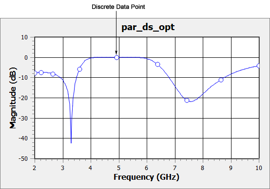
Sonnet graphs show a symbol at each discrete data point. Symbols are not shown for synthesized data points. An example is shown below.
Analysis Issues
There are several issues of which you should be aware when using the ABS technique. See below for more information.
Progress Bar
Since the total number of frequencies required to reach ABS convergence is not known until the analysis has finished, the percent complete shown in the Job Queue's progress bar while the analysis is running is only an estimate.

Multiple Box Resonances
ABS works best when your circuit does not have any box resonances. When your circuit contains box resonances, the ABS algorithm will produce accurate results but may require extra discrete data points around the resonance. For circuits with many box resonances, it may be more efficient to simulate with a different sweep type. See Box Resonances for a detailed discussion of box resonances.
De-embedding
For an ABS Sweep, if you run with de-embedding enabled, de-embedded data is available for the whole band, but non-de-embedded data is available only for the discrete data points at which full analyses were performed while synthesizing the response. If you wish to have non-de-embedded data for the whole frequency band, you must perform an ABS Sweep with the de-embed option disabled.
For more information about de-embedding, see De-embedding Overview.
Transmission Line Parameters
As part of the de-embedding process, the EM solver also calculates the transmission line parameters, Z0 and Eeff (see Z0 and Eeff). When running an ABS analysis, these parameters are only calculated for the discrete data points at which a full analysis is run. If you need the transmission line parameters at more data points, analyze the circuit using a non-ABS sweep.
Current Density Data
For an ABS Sweep with Compute currents enabled, the current density data is only calculated for the discrete data points. If you wish to calculate the current density data at more points in your band, analyze your circuit using a non-ABS sweep. Since computing current density often requires more analysis time, you may wish to set up two Sweep Sets, a non-ABS sweep at the key frequencies with Compute Currents enabled, and an ABS sweep without current density enabled using an Override. See Mixing ABS and non-ABS Sweeps.
Ripple in ABS S-Parameters
When the value of the S-parameters at discrete data points is close to 1.0 (0.0 dB) over the entire band you may notice small ripples or oscillations in the S-parameter values. This is due to the rational fitting model having too many degrees of freedom when trying to fit a straight line. If this is a problem, it is recommended that you analyze the frequency band in which this occurs with a non-ABS sweep.
Mixing ABS and non-ABS Sweeps
You may also mix ABS with non-ABS sweeps. There are several reasons why you may want to do this:
- You may want to compute current density data at key frequencies but not at all the discrete frequencies required for ABS.
- You may want to view a far field pattern at key frequencies.
- You may want transmission line parameters at key frequencies.
- You may want to perform a full EM analysis at the key frequencies of a filter passband and stopband edges.
- You may wish to control the order of the frequencies analyzed.
For example, if you want to simulate a filter from 4.0 - 8.0 GHz, but you only wish to view current density data at the key frequencies of 5.0, 6.6, and 7.8 GHz, you could set up two Sweep sets as follows:
Enable Compute Currents.
Select Circuit > Settings > [EM Options] and click the Compute Currents checkbox. All Sweep Sets that do not use an override will use this setting.
Add Sweep Set 1.
Add a Frequency List containing 5.0, 6.6, and 7.8 GHz. Since you did not specify an override, the EM solver will compute the current density at these frequencies because the Compute Currents checkbox is selected.
Add Sweep Set 2.
Add an ABS sweep from 4.0 to 8.0 GHz. If you do not specify an override, the EM solver would compute the current density at any discrete frequency points required for the ABS sweep to converge.
Set Sweep Set 2 to not compute currents.
In the second Sweep Set, click the Global Analysis Options icon  , then select the Use local analysis options checkbox and unselect the Compute Currents checkbox as shown below:
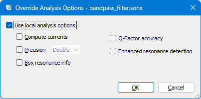
Click OK.
The Options icon changes from the Global Analysis Options icon to the Local Analysis Options icon  . The Analysis Plan should look similar to the picture below.
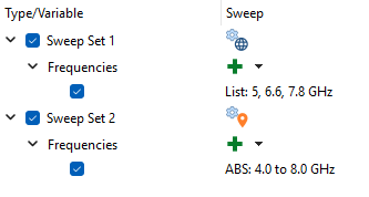
The EM solver will first analyze the three frequencies in Sweep Set 1 and compute the currents. Then, it will perform an ABS sweep from 4.0 to 8.0 GHz without computing the current density.
It is usually recommended to place any discrete frequency sweeps before any ABS sweeps because the ABS sweep will take advantage of the data from the discrete frequencies, allowing it to converge sooner.