Optimization
You may use variables to perform an optimization of your circuit. When you set up an optimization, you specify goals and the range for each variable you wish to allow to vary. The software, using a conjugate gradient method, iterates through multiple variable values, searching for the best set which meets your desired goals.
The Optimizer
The conjugate gradient optimizer begins with analyzing the circuit at the nominal variable values. It then perturbs each variable individually, while holding the others fixed at their nominal values, to determine the gradient of the error function for that variable. Once it has perturbed each variable, it then performs a line search in the direction of decreasing error function for all variables. After some iterations on the line search, the optimizer again calculates the gradients for all variables by perturbing them from their present best values. Following this, a new line search is performed. This continues until one of three conditions are met:
- The error goes to zero.
- The error after the present line search is no better than the error from the previous line search.
- The maximum number of iterations is reached.
When one of these three conditions is met, the optimizer stops.
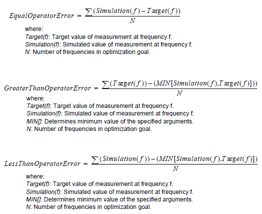
The equations used to determine the optimization goal error are as shown below.
Setting Up an Optimization
Setting up an optimization consists of these steps:
- Setting ranges for the variables you wish to allow to vary
- Specifying your goals, including the frequency range for each goal
- Specifying the maximum number of iterations
The example tune_and_optimization contains projects which have been set up to demonstrate optimization with Sonnet. This example may be accessed using the Example Browser.
Variable Setup
You may choose one or multiple variables to optimize. For each variable that you choose you must specify minimum and maximum bounds, and interpolation settings.
See How to Create a Variable for details on setting up a variable for optimization.
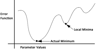
Care should be taken when setting the nominal values for the variables to be optimized. The optimizer starts at the nominal values and converges to the minimum which is closest to those nominal values. Thus, it is highly recommended that you perform some analyses prior to performing the optimization to ensure that the nominal values are in the right value range when the optimizer is started. Otherwise, the optimizer may converge to a local minimum for which the error is not the actual minimum value, as pictured below.
Goal Setup
You specify a goal by identifying a particular measurement and what value you desire it to be. For example dB[S11] < -20 dB. Keep in mind that the goals you specify may not be possible to satisfy. The EM solver finds the solution with the least error.
You may also specify a goal by equating a measurement in one Sonnet project to a measurement in another Sonnet project or data file.
To specify a goal, you must first enable optimization:
Select Circuit > Settings > [Analysis Plan]
The Analysis Plan pane is opened.
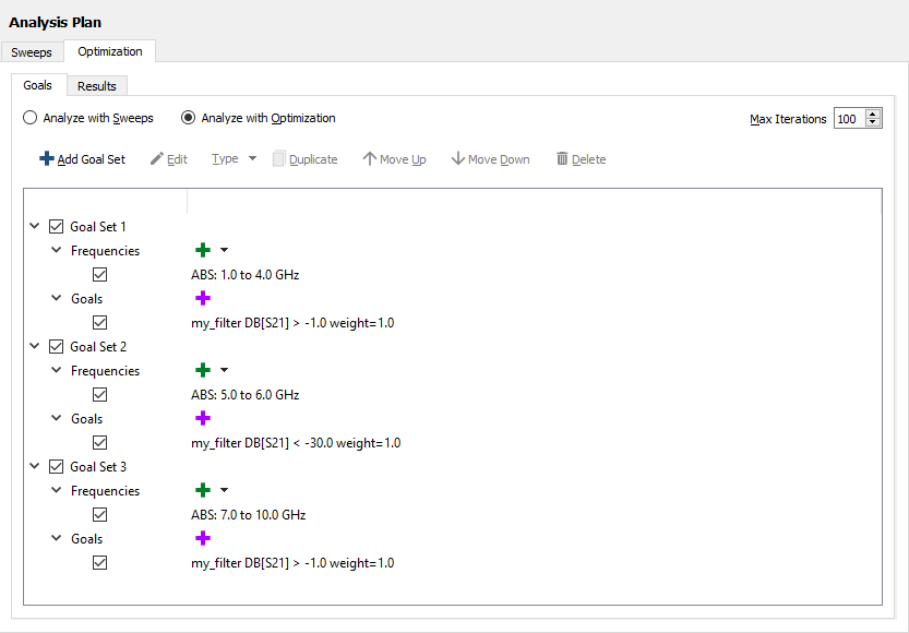
Click the Analyze with Optimization radio button
The Optimization tab is automatically opened. Shown below is the Optimization pane with typical settings.
To specify a goal:
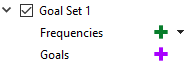
On the Optimization pane, click the Add Goal Set button.
A Goal Set is added to the empty list.
A Goal Set allows you to define a set of frequency sweeps and goals for optimization. A Goal Set may contain a single or multiple goals, all with the same frequency specification. If you need a goal with a different frequency specification, you will need to create another Goal Set.
Click the Add Frequency drop-down list (green plus sign) to add a frequency sweep
The goal will apply to only the frequencies selected. To improve analysis time for the optimization, use as few frequencies as possible. You may add multiple frequency sweeps if you wish. See Sweep Types for an explanation of each type of frequency sweep.
Click the Add Goal icon (purple plus sign) and add your goal.
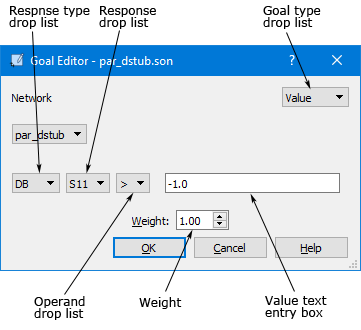 Once you click OK, the goal will be added which will apply to the frequency sweep(s) created in the previous step.
Continue adding goals until you are finished
You may add as many goals as you wish. The error in each goal is multiplied by its Weight. The total error is the weighted sum of all your goals.
Number of Iterations
You specify the maximum number of iterations for your optimization. For each iteration, the EM solver selects a value for each of the variables included in the optimization, then analyzes the circuit at each frequency specified in the goals. Depending on the complexity of the circuit, the number of analysis frequencies and the number of variable combinations, an optimization may take a significant amount of processing time. The number of iterations provides a measure of control over the process. Note that the number of iterations is a maximum. An optimization can stop after fewer iterations if the optimization goal is achieved or it finds a minimum (finds no improvement in the error in further iterations).
Performing an Optimization
To perform an optimization, select Launch > Analyze. You may observe the optimization as it progresses. The initial error as well as the error for the present and best iteration are displayed and updated as the optimization progresses.
You may notice that some iterations complete more quickly than others. This is because the EM solver can reuse portions of the results from previous iterations.
Graphs
You may open a graph tab while the optimization is still running using Launch > Graph Response. This allows you to stop the optimization and start it over using new variable ranges or new goals if the results are not desirable. If you wish to continue viewing data as the optimization runs, select Graph > Refresh.
There are several types of graphs you may wish to create:
- Plot over parameter: Select Graph > Plot Over > Parameter to plot against a parameter. If the parameter is not the one you want, select Graph > Manage Curves and double-click Parameters in the Properties pane and click <Select...>. Then select the desired parameter in the Plot over Variable drop-down list.
- Plot over optimization iteration: Select Graph > Plot Over > Optimization Iteration to plot against the iteration number. This type of graph can give you insight into the progress of your optimization.
- Plot best iteration: Select Graph > Manage Curves and double-click Parameters in the Properties pane and click <Best Opt Error>. Plotting the best iteration will allow you to judge whether or not to use the optimized values of the parameters. If the optimization is still running, you will need to refresh the graph (Graph > Refresh) and choose <Best Opt Error> again since the best parameter combination may have changed.
Accepting the Optimization Results
Once the optimization is complete or you stop the optimization, you have a choice of accepting the best iteration values for the variables resulting from the optimization.
Select Circuit > Settings > [Analysis Plan] from the Project Editor main menu.
If the Optimization tab is not selected, select it.
Click the Results tab.
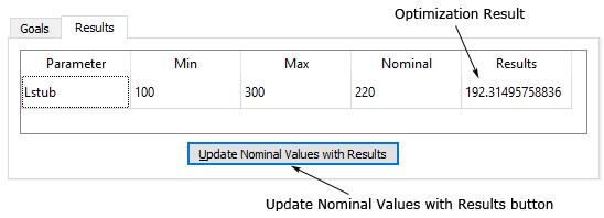
Click the Update Nominal Values with Results button.
The present nominal values of the parameters are replaced with the optimization results.
Click OK and save your project.