Variables

Variables are user-defined circuit attributes that allow the EM solver to modify the circuit in order to perform parameter sweeps and optimization. Also, variables provide a quick way for the user to change dimensions in the Project Editor or multiple elements in a circuit. For example, the length of a transmission line can be assigned the variable L. To change the length of the transmission line, you edit the value for L. Another example would be a circuit which contains 10 resistors, all of which have the same value. Entering a variable R for the resistance of these ideal components allows you to change the value of all 10 resistors by changing the value in only one place. 

A variable’s value may be defined using:

• A constant or nominal value
• Another variable
• An equation

Any of these definitions may be directly entered into a property field.

How to Create a Variable

You may use two basic approaches to creating variables in your project. The first approach is to define all the desired variables and then enter these variables as property values. The second approach is to enter a variable in the desired property field as needed. If the variable has not been previously defined, you are prompted to enter a definition.

To define a variable:

Select Circuit > Settings > [Variables] and click the Add button to open the Add/Edit Variable dialog box.

Alternatively, you may enter an undefined variable in a property field in most dialog boxes. When the dialog box is closed the Add/Edit Variable dialog box is opened. You may also click <Add Variable> from a drop-down list of a property field in most dialog boxes as shown below.

Fill in the fields of the Add/Edit Variable dialog box.

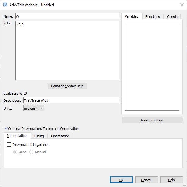
You may hover over any of the fields to see a brief explanation of the field. The value of the variable may be a constant, another variable, or an equation. If you wish to use a pre-existing variable in the equation, you may select it from the list of Variables and click the Insert into Eqn button. The variable name will be entered at the present location of the cursor in the Value text entry box. For information about creating your own equation, see Equations below.

Expand the Optional Interpolation, Tuning and Optimization section

This step is optional. There are three tabs which are explained in more detail below.

Interpolation

The Interpolation tab in the Add/Edit Variable dialog box controls the Interpolation options for the variable being edited or defined.

Interpolate this variable: When interpolation is enabled, a set of values is defined at which the EM solver performs a full electromagnetic simulation. For all other values, it performs a linear interpolation.

When this checkbox is selected, the Auto and Manual radio buttons below are enabled.

• Auto: Clicking this radio button allows the software to automatically determine the values at which a full EM simulation is performed. If a Dimension Parameter is set to an independent variable, the variable’s Resolution will be the cell size and the Reference will be 0.
• Manual: Clicking this radio button allows advanced users to manually control the interpolation of the variable. The Resolution and Reference text entry boxes appear when Manual is selected.
• Resolution: This defines the difference between values at which a full simulation is performed.
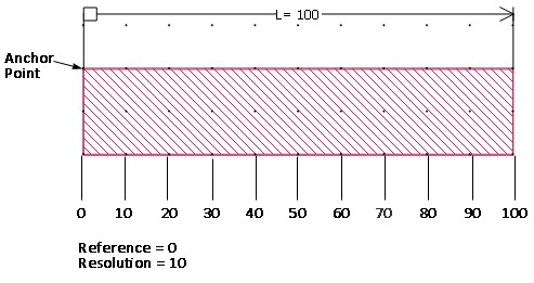
• Reference: This sets the starting point for the set of values at which a full simulation is performed. In the case of Dimension Parameters, this allows you to ensure that the values fall on grid, so that the analysis is as accurate as possible as explained in the example below.

In the example shown below, the cell size is 10 x 10 mils and the variable L is defined as 100 mils. The polygon as entered is directly on grid, so the Anchor Point of the Dimension Parameter falls on grid. For this case, we use a reference of 0. With the resolution set to 10, the values for L would be 10, 20, 30, 40, 50, etc. up until the maximum value.

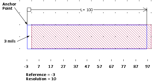
In the second case, shown below, the entered polygon, highlighted in blue, is shifted 3 mils to the left. In this case the Anchor Point is off grid. For this case, we use a reference of -3. With the resolution set to 10, the values for L would be 7, 17, 27, etc. up until the maximum value.

Tuning

The Tuning tab in the Add/Edit Variable dialog box controls the tuning options for the variable being edited or defined.

Allow tuning of this variable: Select this checkbox if you wish to be able to tune this variable in either a Sonnet graph or when using the SEC feature in Sonnet's Keysight ADS Interface. If tuning is enabled, then a slider bar for this variable appears in the Tuning dialog box of a Sonnet graph. This allows you to interactively change the value of the variable and see the effect on your graph. Selecting this checkbox enables the controls listed below:

• Minimum and Maximum: These entries define the data range for the variable while tuning. Enter the lowest and highest values to which the variable may be set while tuning.
• Step: Enter the difference between tuning values in this text entry box. This is the step size used for the slider bar.

Optimization

The Optimization tab in the Add/Edit Variable dialog box controls the optimization options for the variable being edited or defined.

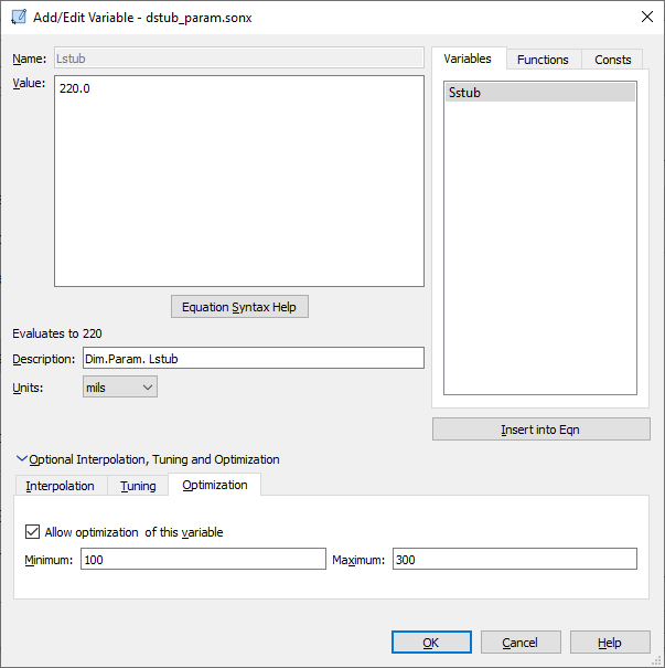
Allow optimization of this variable: Select this checkbox if you wish to be able to use this variable when performing an optimization. When this checkbox is selected, the Minimum and Maximum text entry boxes are enabled. Enter the range of values you wish to allow for the variable during the optimization. For more details, please see the Optimization topic.

Equations

You may enter an equation in any field in which you may enter a variable. A variable may be defined by a constant, another variable or an equation. An equation may be composed of constants, variables and functions. Below are some examples of valid equations.

• 3 * 4.1e-7
• 10.7 * PI
• 6*H 
• sin(theta1)
• sqrt(H)

The last three equations are ones in which one variable is used to define another. This allows you to relate properties in your circuit such that changing one effects the other, maintaining a set relationship between them. For example, if you wish to define a dielectric layer which is always five times the thickness of your substrate, you would define a variable "sub" which you would enter as the thickness of your substrate. Then you would enter "5*sub" as the value for the thickness of the dielectric layer. There are two methods you may use to do this. The first is to define another variable "die_thick" which you define as "5*sub" and the second is to simply enter the equation “5.0 * sub” as the thickness of the dielectric layer.

Variables, Functions, and Constants

The right section of the Add/Edit Variable dialog box contains three tabs. These tabs aid you in creating an equation.

Variables: The Variables tab provides you with a list of variables which you have previously defined. You may double-click the variable name to insert it into the Value box at your present cursor location. Alternatively, you may select the variable name and click the Insert into Eqn button.

Functions: The Functions tab lists all of the available math functions and operators that you may use in your equations. Functions are case sensitive.If you select any function, and then click the Insert into Eqn button, the selected function is automatically copied into the Value box at your present cursor location.

If you hover your cursor over a function, a tooltip pops up with a brief description of the function.

Consts: The Consts tab lists all of the built-in constants that you may use in your equations. If you select any constant, and then click the Insert into Eqn button, the selected constant is automatically copied into the Value box at your present cursor location.

If you hover your cursor over a constant, a tooltip pops up with a brief description of the constant.

Frequency Dependency

The keyword FREQ is available for use in Sonnet equations. This allows you to model properties whose characteristics are frequency dependent such as a dielectric constant. The units of FREQ are Hertz.

Temperature Dependency

The keyword TEMP is available for use in Sonnet equations. This allows you to model properties whose characteristics are temperature dependent such as a conductor conductivity. See Temperature Dependency for details on setting temperature coefficients for conductors. The units of TEMP are degrees Celsius.

Table Functions

The table1 and table2 functions allow you to define an equation that obtains its values from an external file.

table1

Syntax: table1("filename.csv", <key>)

• "filename.csv": The path of a comma-separated value (.csv) file. If only the file name is specified (with no path), then the file should be in the same directory as the source project. You may also use relative paths. Double-quotes are required.
• <key>: The value from the first column of the desired entry in the external file. The function returns the second value. If the <key> value does not occur in the file, then linear interpolation of the file is used to return a value. Note that you may not extrapolate; the <key> value must fall between two existing values in the table.
  
  The key value does not need to be a fixed number; you may use the constant FREQ or a variable as key values. For example, you may define a variable as table1("example.csv", FREQ) which would define a variable which changes with the frequency according to the numbers in the table "example.csv". Please note that the frequency units are in Hz.

The external file should be composed of two columns of data. The first column is the key, and the second is the value. The values should be separated by commas. Comments should be preceded by an exclamation point (!). The exclamation point may be the first character on a line or occur later on the line.

For example, the file example.csv could contain the following entries:

! Project galaxy data

1, 45

3, 135

7, 315 !My comment

8, 360

The following shows the results of using a table1 function for this example:

table1("example.csv", 3) = 135

table1("example.csv", 4) = 180

table1("example.csv", 8) = 360

table2

While the table1 function allows you to have only one value per key, the table2 function allows you to define a row of multiple values, and use the two keys to identify a specific value in the row.

Syntax: table2("filename.csv", <rowkey>, <colkey>)

• "filename.csv": The path of a comma-separated value (.csv) file. If only the file name is specified (with no path), then the file should be in the same directory as the source project. You may also use relative paths. Double-quotes are required.
• <rowkey>: The row number from which you wish to obtain a value.
• <colkey>: identifies the column from which you wish to obtain the value.

The function returns the value from the specified row/column in the source file.

If the <rowkey> or <colkey> does not occur in the file, then interpolation of the file is used to return a value. The key values do not have to be fixed numbers; you may use the constant FREQ or a variable as key values.

The external file should be composed of a matrix of data separated by commas. Comments should be preceded by an exclamation point (!). The exclamation point may be the first character on a line or occur later on the line.

For example, the file "table2d.csv" could contain the following entries:

! Project galaxy data

 ,  1, 2, 3, 4, 5,  6

 2, 2, 4, 6, 9, 10, 12

 4, 4, 8,12,16, 20, 24

 6, 6,12,18,24, 30, 36

 8, 8,16,24,32, 40, 48

10,10,20,30,40, 50, 60

12,12,24,36,48, 60, 72 !My comment

14,14,28,42,56, 70, 84

16,16,32,48,64, 80, 96

18,18,36,54,72, 90,108

20,20,40,60,80,100,120

22,22,44,66,88,110,132

Note the comma at the beginning of the first line. It is not required by Sonnet, but if that comma is not present, many spreadsheet programs, such as Microsoft Excel, may not parse the file. On the other hand, Excel allows a dummy value before that first comma which is not accepted by Sonnet. Extra spaces are permitted.

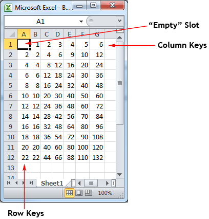
Line 1 is the list of column keys. All other lines are <rowkey> followed by the values in each column. Note that there is no value in the first position in the first line. This is an "empty" slot as it is the intersection of the row and column keys. The external file is displayed below in Excel to more clearly illustrate the format.

The following shows the results of using a table2 function for this example:

table2("table2d.csv", 2,4) = 9

table2("table2d.csv", 8,1) = 8

table2("table2d.csv", 16,3) = 48

table2("table2d.csv", 15.2,3.5) = 53.2

Dependent Variables

One variable is dependent upon another if the value of the variable is defined by an equation that uses another variable. As the value of the variable in the equation is changed, so is the dependent variable. If a variable is dependent, you may not directly edit its nominal value; instead, you change its value by changing the value of the variable on which it is dependent. Variables which do not depend on another variable for their value are independent variables. Only independent variables may be selected for a parameter sweep. To vary a dependent variable in a parameter sweep, you must select the variable on which it depends.

Circular Dependencies

Care should be taken when creating dependent variables that they do not form a circular dependency. A circular dependency is formed when two variables are dependent on each other. This can happen for two variables or multiple variables. In the case of multiple variables, the dependency extends from the first variable through all the variables until the first variable is dependent upon the last.

An example of a circular dependency would be the two equations A=2*B and B=sin(A). If the Project Editor detects a circular dependency, an error message appears.

Example

The following equation illustrates how the skin depth of a metal conductor may be computed in the Sonnet Project Editor. Here, Sigma is the metal conductivity in Siemens per meter. FREQ represents the frequency in Hertz. TWO_PI and MU_0 are pre-defined constants, provided by Sonnet, representing 2.0* π, and the permeability of free space, respectively. The computed skin depth is in meters. In the Sonnet Project Editor, the procedure is to define the Name and Value of one or more variables. In the example, we have a variable named "Sigma" with a value of 4.09e7, and a second variable named "SkinDepth" with the value returned by the square root function.

Sigma = 4.09e7

SkinDepth = sqrt ( 2.0 / (TWO_PI * FREQ * MU_0 * Sigma) )

---