Far Field Patterns - Overview
The Far Field Viewer feature is only available if you have purchased a Far Field Viewer license from Sonnet. The Far Field Viewer license is an optional add-on to Sonnet Suites and must be purchased separately.
The Far Field Viewer calculates and plots far field antenna patterns of a Sonnet project. After an EM simulation is complete, you may display a far field pattern of your antenna. The pattern is based on the current distribution data generated by the EM solver. To generate the current distribution data, enable the Compute currents option (Circuit > Settings > [EM Options]) in your project prior to analysis.
The accuracy of the Far Field Viewer data relies on the accuracy of the EM simulation. Please see Antennas and Radiation for tips on obtaining an accurate EM simulation.
Although the current data is calculated in the EM solver within a metal Analysis Box, the box is removed for the Far Field calculations.
Far Field Viewer Limitations
The Far Field Viewer has the following limitations:
- The plotted antenna patterns use data before de-embedding has been applied. Therefore, the effect of the port discontinuity and any metal that is negated by de-embedding is still included even if you specify de-embedding in your project.
- Radiation from triangular subsections is not included (see Diagonal Edges).
- The calculations assume the dielectrics extend to infinity in the lateral dimensions.
Opening a Far Field Pattern Tab
There are several ways to open a Far Field Pattern tab:
- Click the Plot Far Field button
 from the Session tab.
 - Select File > Plot Far Field Pattern from the main menu in the Session tab.
- Select Launch > Plot Far Field Pattern from the main menu of any other tab in your Session.
- Select File > Open from an existing Pattern tab.
- On Windows systems right-click on a Sonnet project file in File Explorer, then select View Far Field from the pop-up menu which appears.
By default, a polar plot is opened when the Far Field Pattern tab is first opened. You may open a Cartesian or 3D pattern tab by clicking on the Cartesian button  or 3D View button
  . You may also change your Initial Graph Type by selecting Edit > Preferences > [New Graph].
Calculations Setup
When you first open a Pattern tab, a Calculations Setup dialog box appears. To plot a pattern, you must pre-calculate a collection of pattern data. You may only plot patterns that use data from the collection. You may add, remove, or edit pattern data in the collection using the tabs in the Calculations Setup dialog box.
2D Patterns: The Calculations Setup dialog box contains three or four tabs: Frequencies, Angles, Ports, and Parameters (if your project uses parameters). Click the appropriate tab to add, remove or edit data. Adding frequencies and parameter combinations will automatically add curves to your plot when you click the Calculate button.
3D Patterns: The Calculations Setup dialog box contains two or three tabs: Frequencies, Ports, and Parameters (if your project uses parameters). Click the appropriate tab to edit your data. When you click the Calculate button, Sonnet will recalculate the far field data and update your pattern.
You may edit your collection at any time by returning to this dialog box by selecting Graph > Calculations or clicking the Calculations button ![]() .
.
See 2D Patterns or 3D Patterns for details on customizing your antenna pattern.
Spherical Coordinate System
To view a polar or Cartesian antenna pattern, the Far Field Viewer uses the spherical coordinate system shown below. The X, Y, and Z coordinates are those used in the EM solver and the Project Editor. The XY plane is the plane of your Project Editor window, with the Z-axis pointing toward the top cover of the Analysis Box. The spherical coordinate system uses theta (θ) and phi (ϕ) as shown in the figure below.
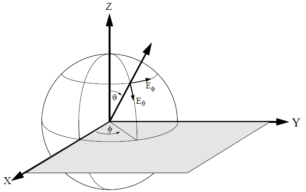 This spherical coordinate system allows values for theta from 0 to 180 degrees. However, values of theta greater than 90 degrees are below the horizon, and are only useful for antennas without infinite ground planes. To view the top hemisphere, sweep theta from 0 to 90 degrees and sweep phi from -180 to +180 degrees.
To view an E-plane cut or an H-plane cut, set phi to 0 or 90 degrees, and sweep theta from -90 to 90 degrees. To view an azimuthal plot, set theta to a positive angle and sweep phi.
You may plot two types of 2D patterns: Cartesian and polar. Both types of plots are shown below. The Cartesian plot is a rectangular graph with your choice of theta, phi, frequency or a parameter for the X-axis. The polar plot allows you to select either theta or phi for the angle axis. Select Graph > Plot Over to change the X-axis or angle axis.

Save to a File
You may wish to save your pattern to a file for future use. The following options are available to you.
Save a Pattern File
Select File > Save or File > Save As to save the presently displayed pattern to a file. The default file name is the base name of the first project displayed with the extension .sptx. To open a pattern file, select File > Open. You may also select File > Add to Graph to add a project to your existing graph. Note that the pattern file only contains information on what is plotted, including the calculations required, but does not include the project files with the analysis results. When you open the pattern file, the referenced projects must exist in the same relative path as they were when the file was saved.
Export Curves to a Spreadsheet
You can export the data from the curves on a 2D far field pattern to a text file, in the form of comma-separated values (CSV), suitable for importing into a spreadsheet. Select Output > All Curves to Spreadsheet from the main menu of a 2D pattern to export the data contained within all the curves on your graph.
Export an Image
Select File > Export Image to save an image of your presently displayed 2D or 3D pattern. The image is stored in Portable Network Graphic (PNG) format.