Subsectioning
Introduction
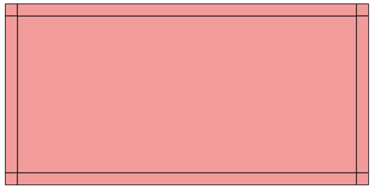
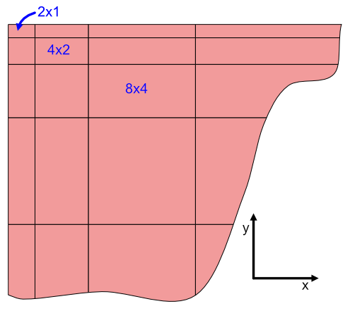
Sonnet's subsectioning is based on a rectangular unit called a cell. One or more cells are automatically combined together to create subsections. Cells may be square or rectangular (any aspect ratio), but must be a consistent size over your entire circuit. When viewed in the Sonnet Project Editor, a cell is represented by the small dots in the Project Editor window. The small dots are placed at the corners of each Cell forming an analysis "grid".
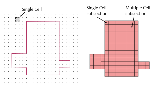
A metal polygon with the cell grid is shown on the left. The same metal polygon’s subsectioning is shown on the right. Note that some subsections are comprised of only one cell, while other subsections are made up of multiple cells.
To set your cell size using the Sonnet Project Editor, select Circuit > Settings > Box from the Project Editor main menu.
If the dots representing the cells are very close to each other, the grid is automatically hidden from view. To see the grid, zoom into an area.
Since multiple cells are combined together to form a single subsection, the total number of subsections is usually considerably smaller than the total number of cells. This is important because the analysis solves an N x N matrix where N is the number of subsections. A small reduction in the value of N results in a large reduction in analysis time and memory.
All EM simulators have an inherent trade-off between speed and accuracy. Decreasing the cell size typically increases the accuracy, but also causes an increase in analysis time.
By default, the EM solver automatically places small subsections in critical areas such as edges where current density is changing rapidly, but allows larger subsections in less critical areas, where current density is smooth or changing slowly. However, in some cases you may wish to modify the automatic algorithm because you want a faster, less accurate solution, or a slower, more accurate solution than is provided by the automatic algorithm.
The following sections explain how the EM solver combines cells into subsections and how you can control this process to obtain an analysis time or the level of accuracy you require.
Snapped Fill
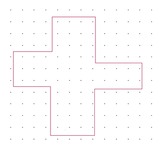
By default, the Sonnet Project Editor displays polygons with an outline and a Snapped Fill pattern. The outline represents the exact geometry that you entered or imported. The Snapped Fill represents the actual subsections analyzed by the EM solver. When the polygon is not aligned with the grid, the actual subsections analyzed by the EM solver may differ from the input geometry as illustrated below.
Snapped Fill off
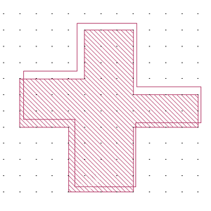
Snapped Fill on
You turn the Snapped Fill on and off by selecting View > Polygon Fill > Snapped Fill and View > Polygon Fill > No Fill in the Project Editor. See Polygon Fill for details and for additional viewing options.
Tips for Determining a Good Cell Size
Selecting a good cell size is key to obtaining an accurate and efficient simulation. The following discussion describes how to select a good cell size.
Find a common factor of your most critical dimensions.
Since your circuit geometry will be snapped to the nearest cell when simulated, you should set your cell size to be a common factor of your most critical dimensions. For example, if your circuit has dimensions of 30 microns, 40 microns and 60 microns, possible cell sizes are 10 microns, 5 microns, 2.5 microns, 2 microns, etc. Large cell sizes result in more efficient analyses, so 10 microns is best if analysis time is an issue.
For complex layouts, the largest common factor that exactly matches all your dimensions may be too small to be practical. In such cases, you should use the Cell Size Calculator to determine the optimal cell size based on your most critical dimensions. This calculator is accessed using the Sonnet Project Editor and selecting Circuit > Settings > [Box]. You input your most critical dimensions into the calculator and specify a tolerance for each value. Then the calculator suggests an optimal cell size. The X and Y dimensions are treated separately. When you are satisfied with the cell size, you may close the calculator, and the cell size is updated.
Calculate the X cell size and the Y cell size independently.
The X cell size and Y cell size do not have to be the same value. Calculate the X cell size based on your dimensions in the X direction, and your Y cell size based on your dimensions in the Y direction.
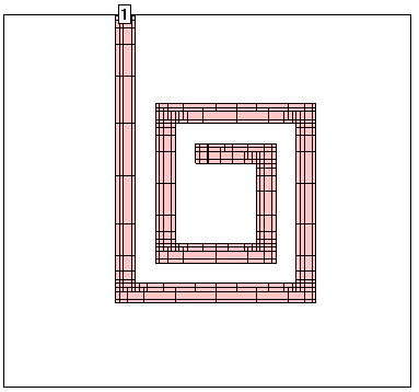
Visually inspect the Snapped Fill (indicated by the fill pattern) for potential problems.
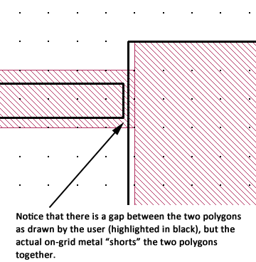
Once a common factor is found, some of your less critical dimensions may not be a multiple of this factor. You should inspect the of your circuit using the Sonnet Project Editor to determine if there are any unintended open or short circuits. You can also use the Connectivity Checker. An example of an unintended short circuit is shown below.
Adjust your cell size for the level of accuracy you require.
A smaller cell size results in a more accurate but slower simulation. Thus, there is a trade-off between speed and accuracy. The accuracy for most circuits will be a function of the number of cells across the width of the transmission lines in your circuit. The more cells across the width, the more accurate the results. For example, a transmission line which is only one or two cells wide results in an error in the characteristic impedance of about 5-6%. For smaller cell sizes, the following equation [3] can be used.
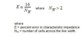
The Sonnet example, Stripline Benchmarks, includes a spreadsheet and Sonnet project files which were used to verify the above equation.
Notice that for NW > 2, each time you halve your cell size, the error is also halved. For example, suppose you chose a cell size of 6.0 microns and your narrowest line width is 12.0 microns. This means your narrowest line will be two cells across the width, resulting in 5-6% error in Z0. Based on the above equation, changing your cell size from 6.0 microns to 3.0 microns (four cells across the line width) results in about 4% error in Z0. You could decrease your cell size even further to 2.0 microns which would decrease your error to about 2%.
Select a cell size that is smaller than 1/20 of a wavelength at the highest simulation frequency.
Most circuits require that your cell size be 1/20 of a wavelength or smaller at all simulation frequencies. Larger cell sizes usually result in unacceptable errors due to incorrect modeling of the distributed effects across the circuit. The EM solver will issue a warning if your cell size is larger than 1/20 of a wavelength at your highest frequency. However, you may wish to calculate this value yourself before you analyze your circuit. If you do, estimate your effective dielectric constant when calculating a wavelength or use the highest dielectric constant in your circuit.
Viewing Subsections
Once you have finished specifying your circuit, you may check how much memory your analysis requires before you run your simulation by selecting Circuit > Estimate Memory.
A pop-up appears to indicate that the circuit is being subsectioned. When the subsectioning is complete, the estimated memory requirement and additional statistics appears in the dialog box. You should ensure that your computer has at least as much RAM as the estimated memory requirement.
You may also view the actual subsections by clicking the View Subsections button. This displays the subsections for your circuit using your present settings, including your cell size. Viewing the subsections can often help determine how to reduce the number of subsections by looking for areas that have dense meshing.
The subsection view is a current density plot with the currents set to zero and the Mesh Type option selected. Therefore, some menus and options in a subsection view may not be applicable to a subsection view.
Meshing Models
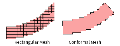
Sonnet offers two techniques to combine cells into subsections: Rectangular Mesh, and Conformal Mesh.
Rectangular Mesh: Uses subsections which are parallel to the Sonnet Analysis Box walls and can have a linear current gradient in the x and/or y direction.
Conformal Mesh: The subsection shape and orientation follows the underlying polygon. This is more efficient for polygons with a curved or irregular shape. However, Conformal Mesh can only be applied to polygons which are transmission-line-like, i.e. the width is small compared to the wavelength. See the Conformal Mesh section for more information.
The picture below shows an example of a sample polygon which is meshed using each technique.
Some of the settings discussed below affect only Rectangular Mesh or only Conformal Mesh and others affect both. Those settings which only affect one of the meshing models are indicated in the descriptions below.
Project Settings
There are multiple ways you can control the subsectioning of your circuit. This section describes settings which affect your entire project. Later sections discuss how to control individual Tech Layers and individual polygons.
All of the project settings are found under Circuit > Settings > [EM Options] in the Project Editor. Some may require you to click the Advanced Subsectioning tab.
Speed/Memory Control
The Speed/Memory control allows you to control the memory usage for an analysis by controlling the Rectangular Meshing for your circuit. The higher memory settings produce a more accurate result and usually increase processing time. Conversely, lower memory settings run faster but usually yield a less accurate result. To access the Speed/Memory control in the Project Editor, select Circuit > Settings > [EM Options].
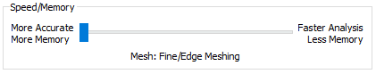
There are three settings for the Speed/Memory control. The default option is Fine/Edge Meshing and is described in Default Subsectioning. An example is shown below. This setting provides the most accurate results but demands the highest memory and processing time.
The second option is Coarse/Edge Meshing. This setting is often a good compromise between speed and accuracy. Shown below is a typical circuit with this setting. Notice the edges of the polygons have small subsections, but the inner portions of the polygons have very large subsections This is often a good compromise between speed and accuracy because the currents on most RF traces change most rapidly on the metal edge.
The last option is Coarse/No Edge Meshing. For this setting, all polygons are set to use large subsections and Edge Mesh is off. This yields the fastest analysis, but is also the least accurate because the modeled current across the width of the line is constant. Shown below is the subsectioning of a typical circuit using this option.
The Speed/Memory controls have no affect on Conformal Mesh subsections.
The following table summarizes the subsectioning parameters used for each of the three Speed/Memory settings. Subsectioning parameters are defined in the Tech Layer Settings section of this page.
| Xmin | Ymin | Xmax | Ymax | Edge Mesh | |
| Fine/Edge Meshing | 1 | 1 | 100 | 100 | On |
| Coarse/Edge Meshing | 50 | 50 | 100 | 100 | On |
| Coarse/No Edge Meshing | 50 | 50 | 100 | 100 | Off |
The Speed/Memory setting overrides any changes to Tech Layer or polygon settings unless it will result in more subsections. For example, setting a Tech Layer's Xmin value to 2 will have no effect if the Speed/Memory control is set to either of the Coarse settings. But if the Xmin value is set to 60, 60 is used because an Xmin of 60 will not result in more subsections. See also Tech Layer Settings and Polygon Settings.
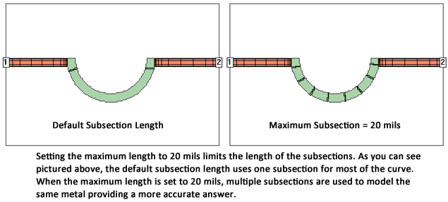
Maximum Subsection Size
The parameter Maximum subsection size allows the specification of a maximum subsection size, in terms of subsections per wavelength. The wavelength is approximated at the beginning of the analysis unless an Estimated epsilon effective is specified. By default, the highest analysis frequency is used for the calculation of the wavelength. This value is a global setting and is applied to the subsectioning of all polygons in your circuit.
The default of 20 subsections per wavelength is fine for most work. This means that the maximum size of a subsection is 18 degrees at the highest frequency of analysis. Increasing this number decreases the maximum subsection size until the limit of 1 subsection = 1 cell is reached.
On rare occasions, you might want to increase this parameter for a more accurate solution. For example, changing it from 20 to 40 decreases the size of the largest subsections by a factor of 2, resulting in a more accurate (but slower) solution. Keep in mind that using smaller subsections in non-critical areas may have very little effect on the accuracy of the analysis while increasing analysis time.
Another reason for using this parameter is when you require extremely smooth current distributions. With the default value of 20, large interior subsections may make the current distribution look choppy. Setting this value to a large number forces all subsections to be only 1 cell wide, providing smooth current distribution. However, analysis time is usually impacted significantly.
Estimated Epsilon Effective
By default, Sonnet uses an automatic algorithm to estimate the effective dielectric constant which is used to determine the wavelength. The wavelength is then used to calculate the Maximum subsection size. You may override the automatic algorithm by entering your own Estimated epsilon effective which forces Sonnet to use your dielectric constant to calculate the wavelength when setting the Maximum subsection size.
Polygon Edge Checking
The Sonnet meshing algorithm attempts to create finer meshing in areas of the circuit where the currents are changing rapidly, and coarser meshing in areas where the currents are relatively constant. When considering the dielectric stackup, it is important for the meshing algorithm to take into account the relative proximity of metal traces located on nearby dielectric layers. The coupling between two metal traces separated by one or more thin dielectric layers can be very strong, thereby necessitating the need for finer meshing in those areas where this coupling is strongest. The Polygon Edge Checking setting controls how far the meshing algorithm looks up and down across dielectric layers when determining where this finer meshing is required.
The default setting is +/- 1 Tech Layer which means the meshing algorithm looks up to the next Tech Layer above the present metal level, and it also looks down to the next Tech Layer below the present metal level. If you were to change this setting to +/- 2 Tech Layers, for example, then the meshing algorithm would look up and down 2 Tech Layers, producing finer meshing in those areas of the circuit where traces separated by 2 Tech Layers couple strongly. The Polygon Edge Checking setting can also be specified in terms of metal levels instead of Tech Layers. Note that entering a value of zero Tech Layers or zero metal levels causes Sonnet to look at the present metal level only.
Subsectioning Frequency
By default, the highest analysis frequency is used to determine the wavelength used in calculating the Maximum subsection size. However, you may change this by entering your own Subsectioning frequency.
Tech Layer Settings
Sonnet provides you with additional meshing controls for an individual Tech Layer. These controls are found in the Meshing Properties section of the Tech Layer Editor. Changes made to a Tech Layer affect all polygons assigned to that Tech Layer. See Polygon Settings for more details.
Controls for Rectangular Mesh are different from Conformal Mesh controls. Rectangular Mesh is covered first, and Conformal Mesh controls are covered later.
Rectangular Mesh
Rectangular Meshing may be controlled using parameters that may be changed for each Tech Layer, allowing you to have coarser resolution for some Tech Layers and finer resolution for others.
These controls are not used for Conformal Mesh subsections. See Conformal Mesh Subsectioning Controls for more details.
Before discussing how to make use of these parameters, we need to first understand Sonnet's automatic subsectioning for a polygon when the parameters are set to their default settings.
Default Subsectioning
The default meshing settings for a Tech Layer are:
- Rectangular Mesh
- Xmin = 1 cell
- Ymin = 1 cell
- Xmax = 100 cells
- Ymax = 100 cells
- Edge Mesh: on
- Include Subsections: X and Y
- Diagonal Edges: Off
The parameters Xmin, Ymin, Xmax, and Ymax specify the smallest and largest allowed size of the subsections in a polygon. With Xmin = 1, the smallest subsection in the X dimension is one cell. With Xmax = 100, subsections are not allowed to go over 100 cells in length.
The illustration below shows how these default subsectioning parameters are used. Notice in the corner, the subsection size is just one cell. The current density changes most rapidly here, thus, the smallest possible subsection size is used.
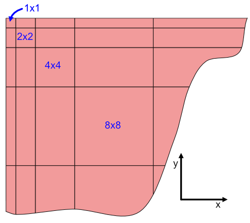
Default subsectioning: Xmin = Ymin = 1, and Xmax = Ymax = 100
As we move away from the corner, along the edge, the subsections become longer. For example, the next subsection is two cells long, the next one is four cells long, doubling each time. If the edge is long enough, the subsection length increases until it reaches Xmax cells, or the Maximum subsection size parameter, whichever comes first, and then remains at that length until it gets close to another corner, discontinuity, etc.
Notice, however, that no matter how long the edge subsection is, it is always one cell wide. This is because Edge Mesh is on. This is the default setting because the current density changes very rapidly on the edge, but becomes smoother on the interior of the metal.
If two polygons butt up against each other or have a small overlap, small subsections will be used at the boundary between the two polygons. Using the Boolean Union command to join the two polygons into one will reduce the number of required subsections. Conversely, if you have an area of your circuit at which you desire greater accuracy, dividing the polygon into two separate polygons at the point of interest will result in smaller subsections in that area.
Xmin and Ymin with Edge Mesh On
In the illustration below, Xmin has been changed to 3. The subsection in the corner is one cell because Edge Mesh is on. The next subsection is 3 cells wide, because Xmin is 3. The next subsection is 6 cells wide, then 12 cells wide, etc., doubling each time.
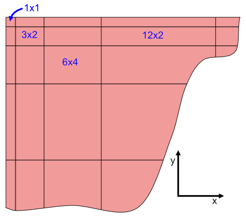
Custom Subsectioning: Xmin = 3, Ymin = 1, and Xmax = Ymax = 100 (Edge Mesh on)
When used in conjunction with large Xmin andYmin values, the Edge Mesh option can be very useful in reducing the number of subsections but still maintaining the edge singularity, as shown in a simple example below. This is very often a good compromise between accuracy and speed.
Xmin and Ymin set to a very large value and Edge Mesh on.
In the case pictured above, Xmin and Ymin are set to be very large, and the frequency is low enough so that the Maximum subsection size parameter corresponds to a subsection size that is larger than the polygon. This is exactly what is being done when you set the Speed/Memory Control to Coarse/Edge Meshing.
Xmin and Ymin with Edge Mesh Off
For Manhattan polygons with Edge Mesh off, Xmin and Ymin set the size of the edge subsections. Turning Edge Mesh off for non-Manhattan polygons has no effect. By default, Xmin and Ymin are 1. This means the edge subsections are 1 cell wide. When Xmin is set to 2, the subsections along vertical edges are now 2 cells wide in the X direction. This reduces the number of subsections and reduces the matrix size for a faster analysis. However, accuracy may also be reduced due to the coarser modeling of the current density near the structure edge or a discontinuity.
Manhattan polygon with Xmin=2 and Ymin=1, and Edge Mesh off
If Xmin or Ymin are greater than your polygon size, the EM solver uses subsections as large as possible to fill the polygon.
Although the Xmin and Ymin parameters are very useful options, it is not a substitute for using a larger cell size. For example, a circuit with a cell size of 10 microns by 10 microns with Xmin = 1 and Ymin =1 runs faster than the same circuit with a cell size of 5 microns by 5 microns with Xmin = 2 and Ymin = 2. Even though the total number of subsections for each circuit may be the same, the EM solver must spend extra time calculating the value for each subsection for the circuit with the smaller cell size.
Using Xmax and Ymax
You may control the maximum subsection size of individual Tech Layers by using the Xmax and Ymax parameters. For example, if Xmax and Ymax are decreased to 1, then all subsections will be one cell. This results in a much larger number of subsections. Thus, this should be done only on small circuits where extremely high accuracy is required or you need a very smooth current density plot.
If the maximum subsection size specified by Xmax or Ymax is larger than the size calculated by the Maximum subsection size parameter, the Maximum subsection size parameter takes priority.
Include just X or Y subsections
The Include Subsections setting determines the orientation of Rectangular subsections created when a polygon is meshed. The default setting is to mesh the polygon in both the X and the Y directions, which in turn, allows current to flow in both the X and Y directions. Under special circumstances you may wish to limit the direction of current flow on a Tech Layer to either the X or Y direction exclusively, and this meshing control allows you to accomplish that.
Diagonal Edges
When a polygon contains diagonal or curved edges, Sonnet will use small rectangular subsections to approximate the edge. This results in an edge that may look like a staircase as shown in the picture below.

For polygons which are multiple cells wide, the error introduced by the staircase edge is relatively small, and can usually be ignored. However, for polygons which are only one cell wide, an open circuit may result. In the picture on the left below, the user's polygon is outlined in black, and the Snapped Fill pattern shows how a Rectangular Mesh results in an open circuit.
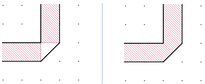
The polygon on the left is set to use Rectangular Mesh without Diagonal Edges enabled, which causes an open circuit since the polygon is only one cell wide. The polygon on the right uses the same cell size, but has Diagonal Edges enabled. This eliminates the open circuit.
To fix this problem, enable Diagonal Edges. This adds triangular subsections on edges of non-Manhattan polygons and removes the open circuit [18].
The Diagonal Edges option places triangular subsections across the diagonal of a cell. In the example above, the triangular subsections corresponded precisely with the polygon's diagonal edge. However, this may not always be the case. For example, in the picture below, the polygon's diagonal edge does not correspond to the diagonal of the cell. The resulting triangular subsection is shown on the right. Notice it does not correspond precisely to the polygon edge, but does still prevent the open circuit caused by the Rectangular Mesh.
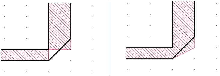
Rectangular Mesh with Diagonal Edges disabled (left) vs. enabled (right) for a polygon with an edge that does not correspond to a diagonal of the cell.
While using triangular subsections on edges can be used to eliminate open circuits, it may increase processing time and should only be used when needed to avoid open circuits.
Conformal Mesh
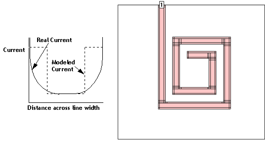
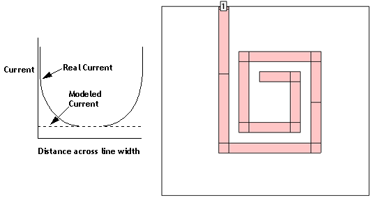
Conformal Mesh is a technique which can dramatically reduce the memory and time required for analysis of a circuit with diagonal or curved transmission lines [19]. Conformal Mesh assumes that most current flows on the edges of circuit conductors, as shown below, and should only be applied when this holds true.
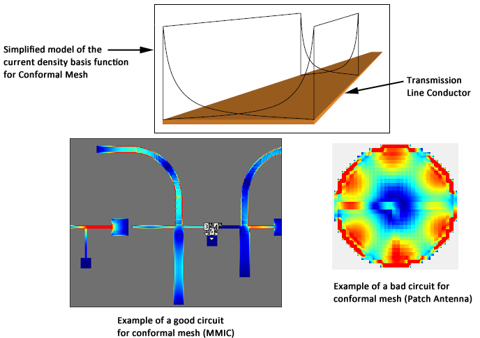
This technique groups together strings of cells following diagonal and curved metal contours to form long subsections along those contours. The illustration below compares the actual meshing of a curved transmission line using Conformal Mesh and Rectangular Mesh. Both have similar accuracy but the Conformal Meshing uses less total subsections, and therefore is more efficient.
Conformal subsections, like Rectangular subsections, are comprised of cells, so that the actual meshing still shows a jagged edge even when the polygon has a smooth edge. However, the Conformal subsections can be much larger. These larger subsections yield faster processing times with lower memory requirements for your analysis.
Rectangular Meshing requires many subsections to model the correct current distribution across the width of a line. Conformal Mesh has this distribution built into the subsection. Sonnet's Conformal Mesh subsections automatically includes the high edge current. This patented capability is unique to Sonnet [20].
Conformal Mesh should be used in places where it will reduce subsection count. For rectangular polygons with no diagonal or curved edges, it is more efficient to use the default Rectangular Meshing. However, if a polygon contains a curved edge, Conformal Mesh provides a quicker analysis without sacrificing accuracy. Conformal Mesh assumes most of the current is flowing parallel to the edge of the Conformal subsection. This works well for transmission lines or geometries that are narrow in one direction with respect to a wavelength.
Conformal Mesh should not be used for geometries like patch antennas and ground planes which have large areas of metal in two directions.
If the polygon is not suitable for Conformal Mesh, then Sonnet may switch portions of the polygon back to Rectangular Mesh.
Cell Size and Processing Time
Care should be taken when choosing your cell size when using Conformal Mesh. Many users, especially experienced Sonnet users, will estimate processing time based on the amount of memory required to analyze a circuit. However, with Conformal Mesh, decreasing the cell size many have only a small affect on the memory required, but could have a much larger affect on analysis time. Therefore, choosing an appropriate cell size is still important.
The significant factor in determining processing time with Conformal Meshing is the number of cells needed to construct a Conformal subsection. The number of Conformal Mesh cells displayed as the result of the Estimate Memory command may be more reliably used as a guideline.
Conformal Mesh Subsectioning Controls
The default length of a Conformal subsection is determined by the Maximum Subsection Size. However, you may reduce this length for an individual Tech Layer by changing the Maximum Length parameter. If this length is less than that determined by the project's Maximum Subsection Size, then Sonnet will use the Maximum Length of the Tech Layer. However, if this length is greater than that determined by the project's Maximum Subsection Size, then Sonnet will use the project's Maximum Subsection Size instead.
Polygon Settings
For a given polygon, you may override its Tech Layer meshing settings. See Inherit vs. Override for more instructions.